|
|
|
|
Fast log-decon with a quasi-Newton solver |
 ,
,  ,
,
 . Set
. Set  .
.
 |
 |
 |
(8) |
 |
|
 |
(9) |
 meets the Wolfe conditions.
 =min
=min ,
,  .
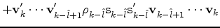
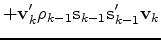
Update
.
Update
 times using the pairs
 ,
i.e., let
,
i.e., let
 and go to 2 if the residual power is not small enough.
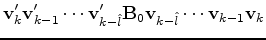
 is not formed explicitly; instead we compute
 with an iterative formula
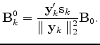
Nocedal (1980). Liu and Nocedal (1989) propose scaling the initial
symmetric positive definite
at each iteration as follows:
is
with an iterative formula
Nocedal (1980). Liu and Nocedal (1989) propose scaling the initial
symmetric positive definite
at each iteration as follows:
is  . In practice, the initial guess
for the Hessian is the identity matrix
. In practice, the initial guess
for the Hessian is the identity matrix  ;
then it might be scaled as proposed in equation (12). The
nonlinear solver as detailed in the previous algorithm converges to
a local minimizer
;
then it might be scaled as proposed in equation (12). The
nonlinear solver as detailed in the previous algorithm converges to
a local minimizer
 of
of
 .
.
|
|
|
|
Fast log-decon with a quasi-Newton solver |