Enhanced interpreter-aided salt-boundary extraction using shape deformation

Mathematical Simplification

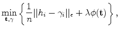
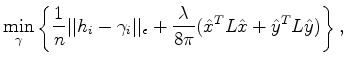
In this section, we reveal more mathematical details of this approach. The actual form of function Q in the objective function 1 is the $\epsilon$ -insensitive L1 norm:

$$\vert\vert v'_i-\mathbf{t}(v_i)\vert\vert _{\epsilon} = \left\{ \... ...t v'_i-\mathbf{t}(v_i)\vert - \epsilon , & \mbox{otherwise} \end{array} \right.$$ (2)

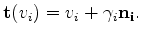
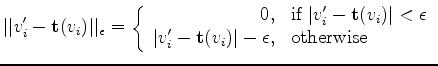
Since new landmark candidates in $V'$ are sought along the contour’s normal direction $\mathbf{n_i}$ , we constrain the desired mapping $\mathbf{t}(V)$ to displace $v_i$ along direction $\mathbf{n_i}$ as well:

$$\mathbf{t}(v_i) = v_i + \gamma_i \mathbf{n_i}.$$ (3)

Let $\gamma = {\gamma_i:i=1,...,n}$ . Since points in $V'$ are found along the normal directions of the original contour $V$ as well, we have $v'_i = v_i + h_i \mathbf{n_i}$ . Then the previous problem 1 becomes

$$\min_{\mathbf{t},\gamma} \left\{ \frac{1}{n} \vert\vert h_i - \gamma_i \vert\vert _{\epsilon} + \lambda \phi(\mathbf{t}) \right\},$$ (4)

subject to constraint 3. As for, we choose the so-called bending-energy term, defined as

$$\phi(\mathbf{t}) = \int\int^{+\infty}_{-\infty} (E(f)+E(g))\; dxdy,$$

where

$$E(\bullet) = \left(\frac{\partial^2{ }}{\partial{x}^2} \right)^2 ... ...}^2} \right)^2 + \left(\frac{\partial^2{ }}{\partial{x}\partial{y}} \right)^2.$$

The nice thing about this choice of bending-energy is that we know in advance, given all mappings that satisfy constraint 3, the mapping specified by thin-plate spline interpolation will minimize the bending-energy (Bookstein, 1989). In other words, the solution $\mathbf{t^{*}}$ to the optimization problem 4 must be the thin-plate spline interpolation that maps $\{V:v_i,i=1,...,n\}$ to $\{\mathbf{t}(V):\mathbf{t}(v_i)=v_i+\gamma_i \mathbf{n_i}, i=1,...,n\}$ . Given that $\mathbf{t}$ must be a thin-plate spline interpolation, we can express $\phi{\mathbf(t)}$ with the vector $\gamma$ . Therefore, this variational problem (where the optimization parameters are functions not numbers) turns into a much simpler numerical convex optimization problem. We just need to find the optimal $\gamma$ for the problem below:

$$\min_{\gamma} \left\{ \frac{1}{n} \vert\vert h_i - \gamma_i \vert... ...n} + \frac{\lambda}{8\pi} (\hat{x}^T L \hat{x} + \hat{y}^T L \hat{y}) \right\},$$ (5)

where $\hat{x},\hat{y}$ is the vector representation of the $x$ and $y$ coordinates of the points in set $\mathbf{t}(V)$ , and $L$ is a semi-positive definite matrix defined by known quantities.

Using the standard SVM technique, we can instead solve the dual problem of 5 according to the K.K.T.(Karush-Kuhn-Tucker) conditions. It ends up being a standard quadratic programming problem with both upper and lower bounds.

Enhanced interpreter-aided salt-boundary extraction using shape deformation