Enhanced interpreter-aided salt-boundary extraction using shape deformation

Examples

Fig3-segT-flow
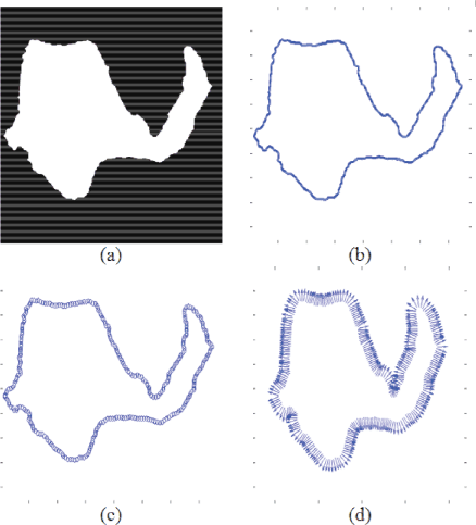
Figure 3. Preprocessing flow on the segmentation result of the template image. (a) Build the salt-body mask. (b) Extract the boundary. (c) Subsample to a list of landmarks. (d) The outnormal directions found for each landmark on the contour.

Fig4,Fig5
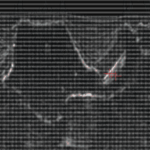
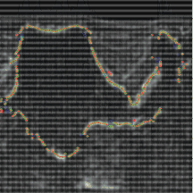
Figure 4. a) The three candidate points found in $B_{137}$ . b) The update of set $V'$ in one iteration. Blue indicates points in $V'$ that are support vector points, red shows the original points in $V'$ , and green shows the updated set $V'$ obtained by replacing the badly fitting points in $v_i'$ with better fitting candidates in $B_i$ .

We test this algorithm on a 3-D seismic image cube from a Gulf of Mexico seismic survey. The cube is of discrete size $970 \times 784 \times 12$ in the depth(Z), inline(X) and cross-line(Y) directions respectively. The grid spacings are $9.6\ensuremath{\, \mathrm{m}}, 25\ensuremath{\, \mathrm{m}}$    and $30\ensuremath{\, \mathrm{m}}$ . We test this algorithm on a 3-D seismic image cube from a Gulf of Mexico seismic survey. The cube is of discrete size $970 \times 784 \times 12$ in the depth(Z), inline(X) and cross-line(Y) directions respectively. The grid spacings are $9.6\ensuremath{\, \mathrm{m}}, 25\ensuremath{\, \mathrm{m}}$    and $30\ensuremath{\, \mathrm{m}}$ . We have only the human-interpreted segmentation result in slice 1, which we use as the template image. We then perform initial processing on this segmentation result to extract the template landmarks as shown in Figure 3.

To find candidates for the set $B_i$ , we overlay the landmark on the energy envelope of the input image (neighboring slice), then we search along the normal direction for certain image features which might suggest that certain locations be part of the boundary. Here we just use a very simple criterion: we choose the locations of the local amplitude maxima as the boundary point candidates. The plot in Figure 4(a) shows all candidates in $B_i$ for $i=137$ .

We then run the optimization for a few iterations. During each iteration, we identify all the support vectors (which correspond to the fitting outliers); for each support vector $h_i$ , we try to use other candidates in set $B_i$ such that the fitting $h_i-\gamma_i$ improves. Figure 4(b) demonstrates this step during one iteration.

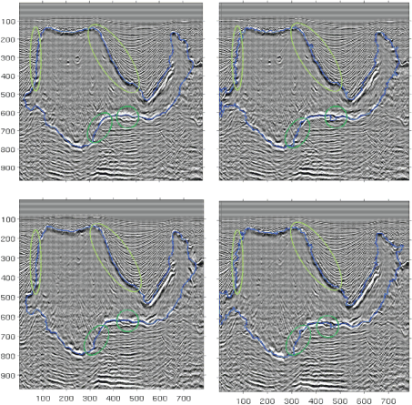
Finally we deform all 12 slices one by one, in increasing distance from the template slice. In Figure 5, we show the comparison between the obtained deformed boundary and the boundary found by automatic methods with the simple way of propagating the user input as described in Halpert et al. (2011). The improvement is prominent, with several regions highlighted in circles. The deformed boundary is less jagged and tracks the local edges in the image better. The shape-preserving constraint helps prevent “boundary leakage” as the automatic segmentation is done using flooding algorithms.

Fig6-segmentComparison
Figure 5. The segmentation result for slices 4 (top) and 12 (bottom) using our boundary deformation technique (left column) and the simple automatic method (right column).

Enhanced interpreter-aided salt-boundary extraction using shape deformation