Residual moveout-based wave-equation migration velocity analysis in 3-D

Extension to 3-D

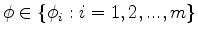
As we shift from 2-D seismic surveys to 3-D ones, two extra dimensions (cross-line axis $y$ and subsurface azimuth $\phi$ ) are added to our seismic image. Therefore we denote the prestack image as $I(z,\gamma,\phi,x,y)$ . Assuming there are $m$ values for $\phi$ , then $\phi \in \{\phi_i:i=1,2,...,m\}$ . Now the maximum-stack-power objective function 1 can be generalized to

$$J(s) = \frac{1}{2} \sum_{x,y}\sum_{z} {\left[\sum_{\phi_i} \sum_{\gamma} \; I(z,\gamma,\phi_i,x,y;s) \right]}^2,$$ (11)

in which we stack the gather along both $\gamma$ and $\phi$ axes.

The next step is to choose a proper residual moveout parameterization for the 3-D ADCIGs, in which the moveout is a surface (defined by $(\gamma ,\phi )$ ) rather than a curve (of $\gamma$ ). There are certainly more than one way to design such parameterization. As an initial attempt, we choose a straightforward approach, in which we separate the moveout surface into individual curves by azimuth $\phi$ . For each azimuth angle $\phi_i$ , we assign the curvature parameter $\rho_i$ and the static shift parameter $\beta$ , respectively. Notice that all the curves share the same $\beta$ parameter, because the center of the move-out surface at ( $\gamma=0,\forall\phi_i$ ) is shared by all curves.

Under this parameterization, the 3-D counterpart of objective function 3 would be

$$J_{Sm}(\rho(s)) = \frac{1}{2} \sum_{x,y} \sum_{z} \sum_{\phi_i}\f... ...um_{z_w} \sum_{\gamma} I^2(z+z_w+\rho_i\tan^2{\gamma},\gamma,\phi_i,x,y,;s_0)},$$ (12)

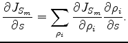
where $\mathbf{\rho}$ becomes a vector, $\rho = \{\rho_i:i=1,2,...,m\}$ . The gradient formula 4 now turns into

$$\frac{\partial{J_{S_{m}}}}{\partial{s}} = \sum_{\rho_i}\frac{\partial{J_{S_{m}}}}{\partial{\rho_i}} \frac{\partial{\rho_i}}{\partial{s}}.$$ (13)

Because each $\phi_i$ is treated separately, we can compute ${\partial{J_{Sm}}}/{\partial{\rho_i}}$ in exactly the same way as we do in the 2-D case.

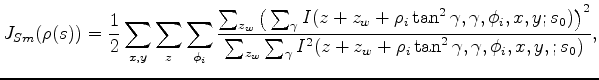
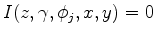
Analogously, we can define an auxiliary objective function for each image point that uncovers the $s \leftrightarrow \rho$ relationship:

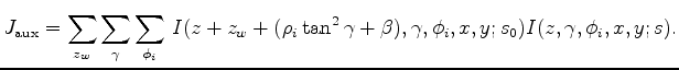$$J_{\mathrm{aux}} = \sum_{z_w} \sum_{\gamma}\sum_{\phi_i} \, I(z+z... ...(\rho_i \tan^2{\gamma} + \beta),\gamma,\phi_i,x,y;s_0)I(z,\gamma,\phi_i,x,y;s).$$ (14)

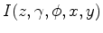
Using the same trick of finding partial derivatives for implicit functions, equation 6 is generalized as

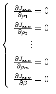$$\renewedcommand{arraystretch}{1.5} \left\{ \begin{array}{c} \frac... ...\ \frac{\partial{J_{\mathrm{aux}}}}{\partial{\beta}} = 0 \end{array} \, \right.$$ (15)

We differentiate equation 15 with respect to $s$ :

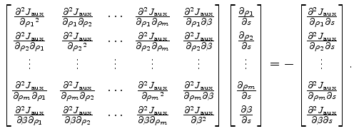$$\renewedcommand{arraystretch}{1.5} \begin{bmatrix}\frac{\partial^... ... \frac{\partial^2{J_{\mathrm{aux}}}}{\partial{\beta}\partial{s}} \end{bmatrix}.$$ (16)

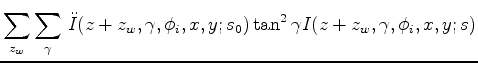
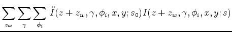
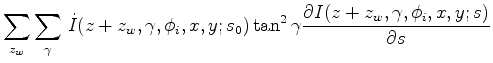
We can calculate the $m+1$ by $m+1$ Jacobian matrix elements and the right-hand side based on equation 14:

$$\frac{\partial^2{J_{\mathrm{aux}}}}{\partial{\rho_i}^2} = \sum_{z_w} \sum_{\gamma} \, \ddot{I}(z+z_w,\gamma,\phi_i,x,y;s_0) \tan^4{\gamma} I(z+z_w,\gamma,\phi_i,x,y;s)$$

$$\frac{\partial^2{J_{\mathrm{aux}}}}{\partial{\rho_i}\partial{\rho_j}} \equiv \; 0 \qquad \qquad \qquad \forall \quad i \ne j$$

$$\frac{\partial^2{J_{\mathrm{aux}}}}{\partial{\rho_i}\partial{\beta}} = \sum_{z_w} \sum_{\gamma} \, \ddot{I}(z+z_w,\gamma,\phi_i,x,y;s_0) \tan^2{\gamma} I(z+z_w,\gamma,\phi_i,x,y;s)$$

$$\frac{\partial^2{J_{\mathrm{aux}}}}{\partial{\beta}^2} = \sum_{z_w} \sum_{\gamma} \sum_{\phi_i} \, \ddot{I}(z+z_w,\gamma,\phi_i,x,y;s_0) I(z+z_w,\gamma,\phi_i,x,y;s)$$

$$\frac{\partial^2{J_{\mathrm{aux}}}}{\partial{\rho_i}\partial{s}} = \sum_{z_w} \sum_{\gamma} \, \dot{I}(z+z_w,\gamma,\phi_i,x,y;s_0) \tan^2{\gamma} \frac{\partial{I(z+z_w,\gamma,\phi_i,x,y;s)}}{\partial{s}}$$

$$\frac{\partial^2{J_{\mathrm{aux}}}}{\partial{\beta}\partial{s}} = \sum_{z_w} \sum_{\gamma} \sum_{\phi_i}\, \dot{I}(z+z_w,\gamma,\phi_i,x,y;s_0) \frac{\partial{I(z+z_w,\gamma,\phi_i,x,y;s)}}{\partial{s}}.$$ (17)

Denoting matrix $\mathbf{F}=\{F_{i,j}\}$ to be the inverse of the Jacobian, then

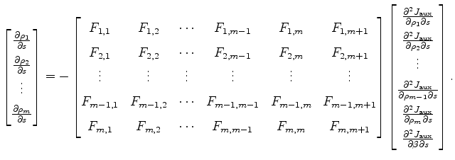$$\renewedcommand{arraystretch}{1.5} \begin{bmatrix}\frac{\partial{... ... \frac{\partial^2{J_{\mathrm{aux}}}}{\partial{\beta}\partial{s}} \end{bmatrix}.$$ (18)

Finally, plugging equation 18 and 17 back into the model gradient expression 13, we get

$$\frac{\partial{J}}{\partial{s}} = -\sum_{z_w} \sum_{\gamma} \sum_... ...partial{s}} (G_{i}\tan^2{\gamma}+G_{m+1}) \dot{I}(z+z_w,\gamma,\phi_i,x,y;s_0),$$ (19)

in which

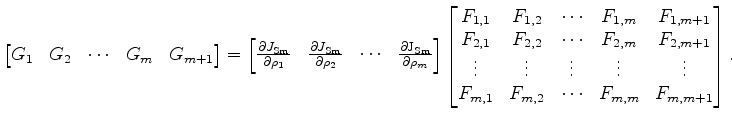$$\begin{bmatrix}G_1 & G_2 & \cdots & G_m & G_{m+1} \end{bmatrix} =... ...ts & \vdots \\ F_{m,1} & F_{m,2} & \cdots & F_{m,m} & F_{m,m+1} \end{bmatrix} .$$ (20)

In practice, there are some caveats when taking the inverse of the Jacobian matrix. The Jacobian can be ill-conditioned when all elements in one row or column are close to zero. For example, if the image point is not illuminated from a certain azimuth direction $\phi_j$ , i.e. $I(z,\gamma,\phi_j,x,y) = 0$ , then the $j_{th}$ row and column of the Jacobian would be zero. In order to avoid numerical overflow under this circumstance, we pre-exclude those azimuth angles with poor illumination energy from the Jacobian, and we invert a subset of the original Jacobian that contains only image gathers at well-illuminated azimuth angles.

Residual moveout-based wave-equation migration velocity analysis in 3-D