|
|
|
|
Residual moveout-based wave-equation migration velocity analysis in 3-D |
In this example, the model is
 in
in  ,
in
,
in  and
and
 in
in  ; the grid sampling is
 in
and
,
in
and
,
 in
.
The receivers are fixed during the entire survey, spanning a rectangular area from
in
.
The receivers are fixed during the entire survey, spanning a rectangular area from
 to
to  with receiver spacing of
in both
and
.
The shot locations cover the same region as the receivers do, and the shot spacing is
with receiver spacing of
in both
and
.
The shot locations cover the same region as the receivers do, and the shot spacing is
 .
This leads to a survey of
.
This leads to a survey of
 receivers and
 shots along both
and
.
A total of 32 frequencies are calculated, ranging from
shots along both
and
.
A total of 32 frequencies are calculated, ranging from
 to
to
 . There is one flat reflector at a depth of
 .
A constant starting velocity of
.
A constant starting velocity of
 is used. The true model is a constant background velocity (
, same as the starting velocity), but with a
width,
is used. The true model is a constant background velocity (
, same as the starting velocity), but with a
width,
 height Gaussian anomaly at the center, with a peak value of
 .
Figure 1 shows the true velocity model.
.
Figure 1 shows the true velocity model.
First, we compute the initial subsurface ODCIG (offset-domain common-image gather) with the offset  range being
 .
The acquisition geometry we use can provide full azimuth for the inner portion of the model. We choose to generate ADCIGs along three azimuth angles:
.
The acquisition geometry we use can provide full azimuth for the inner portion of the model. We choose to generate ADCIGs along three azimuth angles:
 and
and  .
.
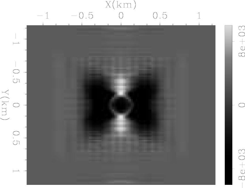
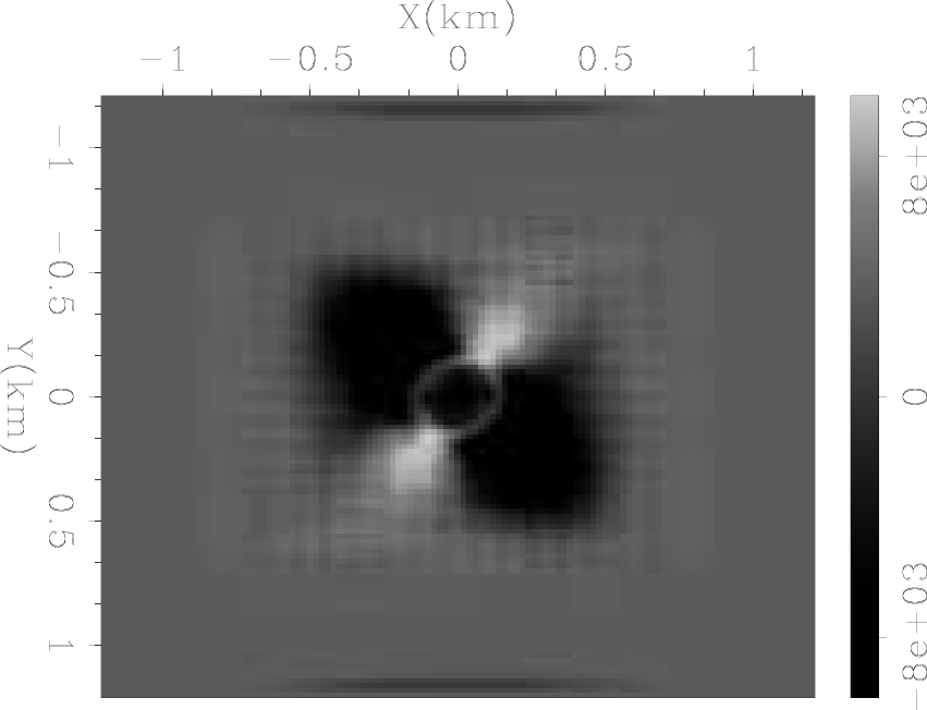
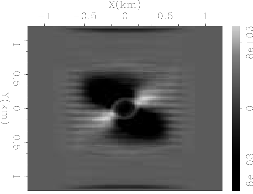
Figure 2 shows the derivatives of the semblance objective function over the moveout parameter  , with each panel representing a distinct azimuth:
 and
and  degrees.
Since the migration velocity is slower than the true one, most of the ADCIGs would be curving upward, therefore a proper objective function should instruct the inversion to decrease the curvature.
Figure 2 verifies the consistency between the numerical result and our theoretical expectation.
Notice in each plot, there are some positive values on the direction perpendicular to the azimuth orientation.
This is caused by the fact that at these locations, the seismic energy traveling through the designated azimuth probes a much smaller anomaly.
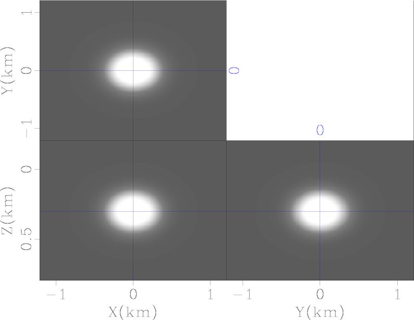
(Imagine we have a spheric anomaly centered around the origin:
degrees.
Since the migration velocity is slower than the true one, most of the ADCIGs would be curving upward, therefore a proper objective function should instruct the inversion to decrease the curvature.
Figure 2 verifies the consistency between the numerical result and our theoretical expectation.
Notice in each plot, there are some positive values on the direction perpendicular to the azimuth orientation.
This is caused by the fact that at these locations, the seismic energy traveling through the designated azimuth probes a much smaller anomaly.
(Imagine we have a spheric anomaly centered around the origin:
 , the strength of the anomaly decreases by distance from the center. If we intercept the anomaly with vertical plane
  , the anomaly seen on the section is strong because the section passes through the center of the sphere. However, if we intercept the sphere with
  , the anomaly seen on that plane would be much weaker and smaller, because the part of the anomaly seen on this plane is far away from the center.)
In this case, the ADCIG at near angles are affected by the anomaly but the far angles are not, therefore showing the opposite curvature.
This phenomenon might hinder the tomography algorithm from finding a good update. Fortunately, with more than one azimuth, the curvatures observed from the alternative azimuth would offset this effect. This example shows one of the advantages of having multiple azimuth image gathers.
, the anomaly seen on that plane would be much weaker and smaller, because the part of the anomaly seen on this plane is far away from the center.)
In this case, the ADCIG at near angles are affected by the anomaly but the far angles are not, therefore showing the opposite curvature.
This phenomenon might hinder the tomography algorithm from finding a good update. Fortunately, with more than one azimuth, the curvatures observed from the alternative azimuth would offset this effect. This example shows one of the advantages of having multiple azimuth image gathers.
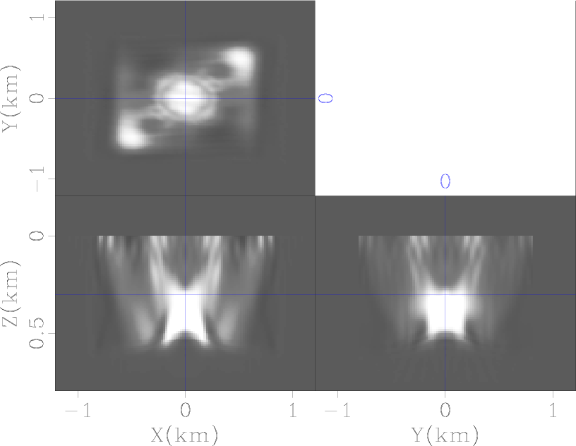
Figure 3 shows the first model gradient (in velocity) calculated using our approach. Qualitatively, the method works as we expected. The update is concentrated around the anomaly's location and the sign of the update is correct.
|
|---|
|
vel3d
Figure 1. The true velocity model, with positive Gaussian anomaly in the center. |
|
|
|
|---|
|
dJdu0,dJdu30,dJdu60
Figure 2. The  term for (a)
 , (b)
, (b)
 and (c)
 . The values correlates well with the curvatures of the ADCIGs at each
  location.
|
|
|
|
|---|
|
grad-gauss
Figure 3. First gradient of the velocity model calculated by our 3-D RMO WEMVA implementation, i.e.  predicted by our WEMVA objective function.
|
|
|
|
|
|
|
Residual moveout-based wave-equation migration velocity analysis in 3-D |