Early-arrival waveform inversion for near-surface velocity and anisotropic parameters: modeling and sensitivity kernel analysis

Naive parametrization

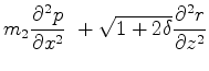
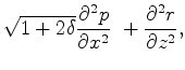
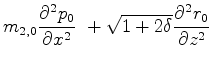
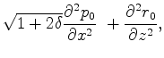
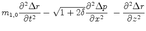
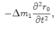
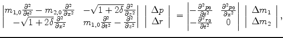
The most naive parametrization directly inverts velocity and ${\epsilon }$ . However, to avoid higher-order term involving both variables, equation 1 can be rewritten as follows:

$$m_1\frac{\partial^2 p}{\partial t^2} = m_2\frac{\partial^2 p}{\partial x^2} \ + \sqrt{1+2\delta}\frac{\partial^2 r}{\partial z^2}$$

$$m_1\frac{\partial^2 r}{\partial t^2} = \sqrt{1+2\delta}\frac{\partial^2 p}{\partial x^2} \ + \frac{\partial^2 r}{\partial z^2},$$ (2)

where ${m_1={v_p}^{-2}}$ and ${m_2={1+2\epsilon}}$ are the two model variables, assuming

$$m_1 = m_{1,0}+\Delta{m_1}$$

$$m_2 = m_{2,0}+\Delta{m_2}$$

$$p = p_0+\Delta{p}$$

$$r = r_0+\Delta{r}$$

$$m_{1,0}\frac{\partial^2 {p_0}}{\partial t^2} = m_{2,0}\frac{\partial^2 {p_0}}{\partial x^2} \ + \sqrt{1+2\delta}\frac{\partial^2 {r_0}}{\partial z^2}$$

$$m_{1_0}\frac{\partial^2 {r_0}}{\partial t^2} = \sqrt{1+2\delta}\frac{\partial^2 {p_0}}{\partial x^2} \ + \frac{\partial^2 {r_0}}{\partial z^2},$$ (3)

By combining this with equation 2, we can obtain

$$m_{1,0}\frac{\partial^2 \Delta{p}}{\partial t^2} - m_{2,0}\frac{\... ...p}}{\partial x^2} \ -\sqrt{1+2\delta}\frac{\partial^2 \Delta{r}}{\partial z^2} = \ -\Delta{m_1}\frac{\partial^2 {p_0}}{\partial t^2} + \Delta{m_2}\frac{\partial^2 {p_0}}{\partial x^2}$$

$$m_{1,0}\frac{\partial^2 \Delta{r}}{\partial t^2} - \sqrt{1+2\delt... ...rtial^2 \Delta{p}}{\partial x^2} \ - \frac{\partial^2 \Delta{r}}{\partial z^2} = \ -\Delta{m_1}\frac{\partial^2 {r_0}}{\partial t^2},$$ (4)

which can be written in the following matrix form:

$$\begin{vmatrix}{ m_{1,0}\frac{\partial^2 }{\partial t^2} - m_{2,0... ...left\vert\begin{array}{c} {\Delta{m_1}} \\ {\Delta{m_2}}\end{array}\right\vert,$$ (5)

This establishes a linear relationship between model perturbation and data perturbation, and can be used to calculate the sensitivity kernel. Figure 5 shows the relative sensitivity kernels of the two model parameters, which are defined as

$$k_{m_i}=g_{m_i}/m_{i,0},$$ (6)

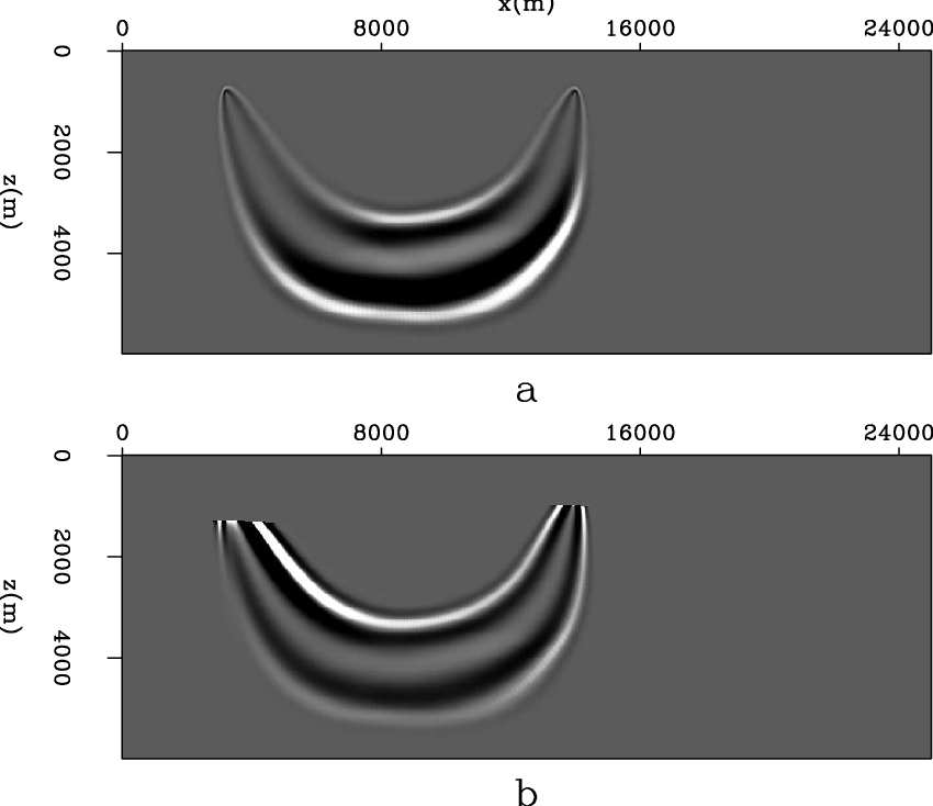
where ${g_{m_i}}$ is the sensitivity kernel, and ${k_{m_i}}$ is the relative sensitivity kernel. the clipping value of the top figure is over sixteen orders of magnitude larger than the bottom figure, which means if we are to use this parametrization for our inversion, there will be almost no updates of the anisotropic parameter.

relimpn
Figure 5. Relative sensitivity kernel of parameter: a) ${{v_p}^{-2}}$ ; b) ${1+2\epsilon }$ . Clipping value of the top figure is ${1e10}$ , clipping value of the bottom figure is ${2e-6}$ .

Early-arrival waveform inversion for near-surface velocity and anisotropic parameters: modeling and sensitivity kernel analysis