|
|
|
|
Early-arrival waveform inversion for near-surface velocity and anisotropic parameters: modeling and sensitivity kernel analysis |
 and
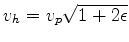
and  are horizontal and vertical stress, respectively,
  is vertical p-wave velocity and
 and
and  are anisotropic parameters (Thomsen, 1986).
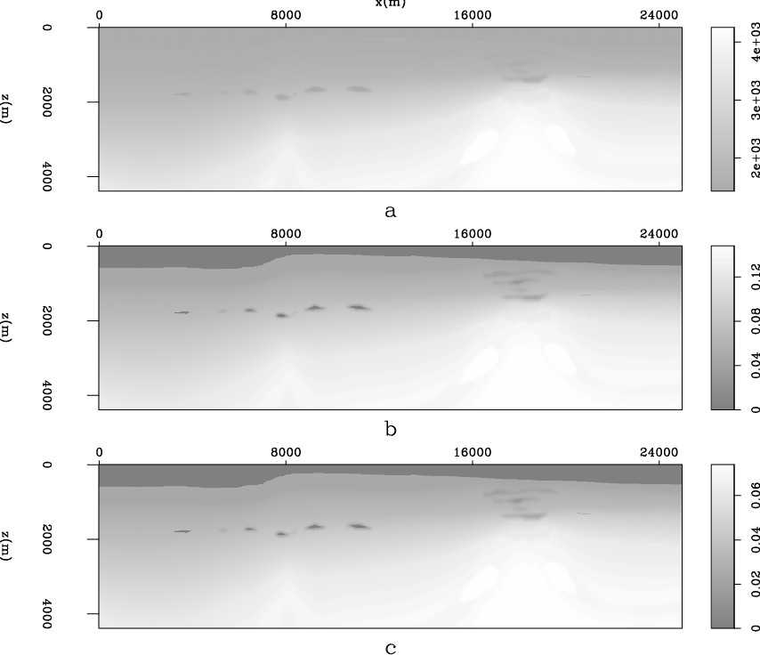
To illustrate the traveltime sensitivity of data to parameter changes, I use part of the BP 2002 benchmark model. The original synthetic model has only p-wave velocity; the anisotropic parameters were created from the velocity model according to typical Gulf of Mexico anisotropic parameters. Velocity,
and
models are shown in Figure 1.
|
|---|
|
modelbw
Figure 1. Reference model for various modeling experiments. Top: velocity model; middle:
model; bottom:
model.
|
|
|
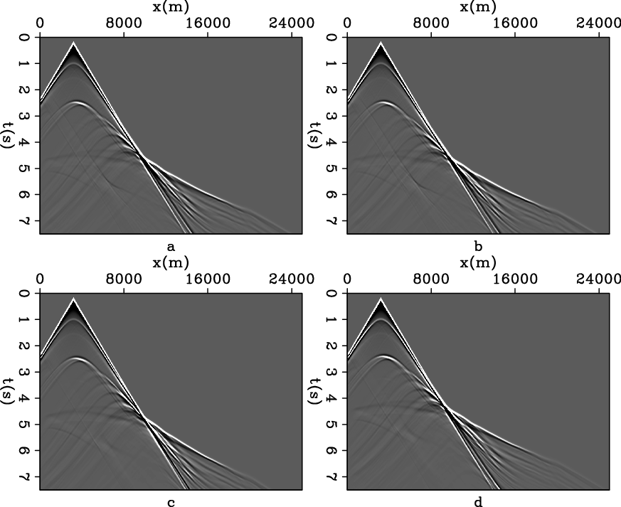
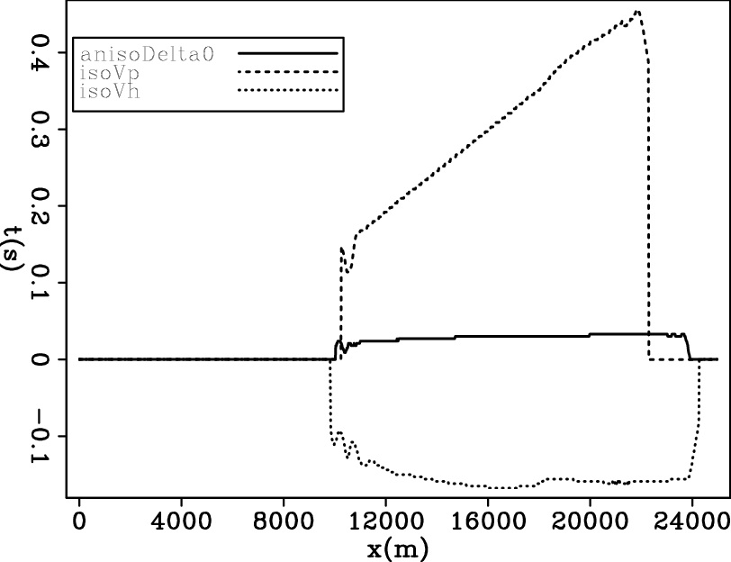
Four different modeling experiments with modeled shot records are shown in Figure 2. The first experiment is the VTI anisotropic modeling using all three fields shown in Figure 1. The second experiment is the same VTI modeling but with
 . The third experiment is isotropic modeling using the velocity field only, and the fourth is isotropic modeling using the horizontal p-wave velocity, which is defined as
 . Figure 3 shows the refraction traveltime difference of the latter three shots compared to the first shot. It can be seen that traveltime is insensitive to
changes, but is sensitive to
changes. Also, isotropic modeling using the horizontal p-wave velocity results in non-trivial traveltime differences, which means that even using isotropic FWI, the retrieved model is not necessarily the horizontal p-wave velocity, as was previously thought (Ghilami et al., 2011).
. Figure 3 shows the refraction traveltime difference of the latter three shots compared to the first shot. It can be seen that traveltime is insensitive to
changes, but is sensitive to
changes. Also, isotropic modeling using the horizontal p-wave velocity results in non-trivial traveltime differences, which means that even using isotropic FWI, the retrieved model is not necessarily the horizontal p-wave velocity, as was previously thought (Ghilami et al., 2011).
|
|---|
|
record
Figure 2. Shots from different modeling experiments: a) VTI modeling using all three fields shown in Figure 1; b) same as a) except that
; c) isotropic modeling using only the velocity field; d) isotropic modeling using horizontal p-wave velocity
.
|
|
|
|
|---|
|
tdif
Figure 3. Refraction traveltime difference of shots compared to the VTI case. |
|
|
|
|
|
|
Early-arrival waveform inversion for near-surface velocity and anisotropic parameters: modeling and sensitivity kernel analysis |