Tomographic full waveform inversion: Practical and computationally feasible approach

Gaussian Model

For the first of synthetic example, we use a two-layer model with a Gaussian anomaly. The velocities for the top layer, bottom layer and peak of the Guassian anomaly are 3000 m/s, 3500 m/s and 3500 m/s, respectively. Figure 1 shows the true velocity model. A Ricker wavelet with a fundamental frequency of 15 Hz and temporal sampling of 1.5 ms is used as a source function to model the data. There are 151 fixed receivers with a spacing of 20 m and 31 sources with a spacing of 100 m. The maximum offset used is 1500 m in both sides and the initial model is a constant model of 3000 m/s velocity.

gauss-true
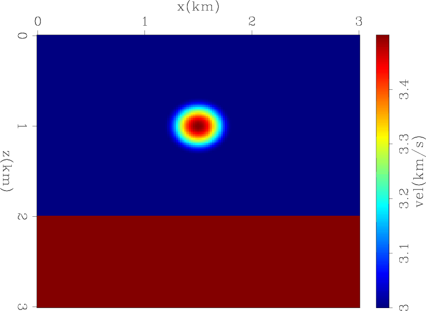
Figure 1. The true velocity of Gaussian model.

We first modeled the observed data with the conventional acoustic wave-equation nonlinear modeling operator. Then, we computed the initial data using the same nonlinear operator on the initial model. The two datasets are subtracted from each other to remove the direct arrivals. We then use the subtracted data as the ``observed data" in equation 10.

gauss-res Figure 2. The data residual norm as a function of iterations of Gaussian model inversion.

We show the results of running 400 iterations of minimizing equation 10 with and without the scale mixing described in equations 16 and 17. Figure 2 shows the normalized residual of the data fitting part, described by the first term of equation 10, as a function of iterations. The residuals of both inversions decrease monotonically without getting stuck in a local minima. However, scale mixing shows a much faster convergence rate.

gauss-imodel
Figure 3. The inverted background of the Gaussian model example.

gauss-imodelr
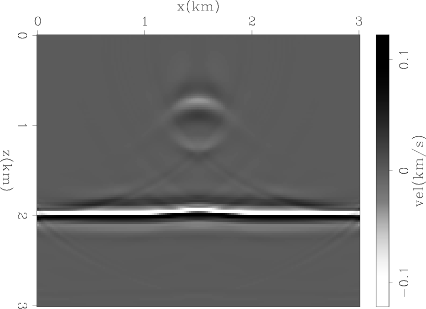
Figure 4. The inverted reflectivity of the Gaussian model example.

gauss-imodel2
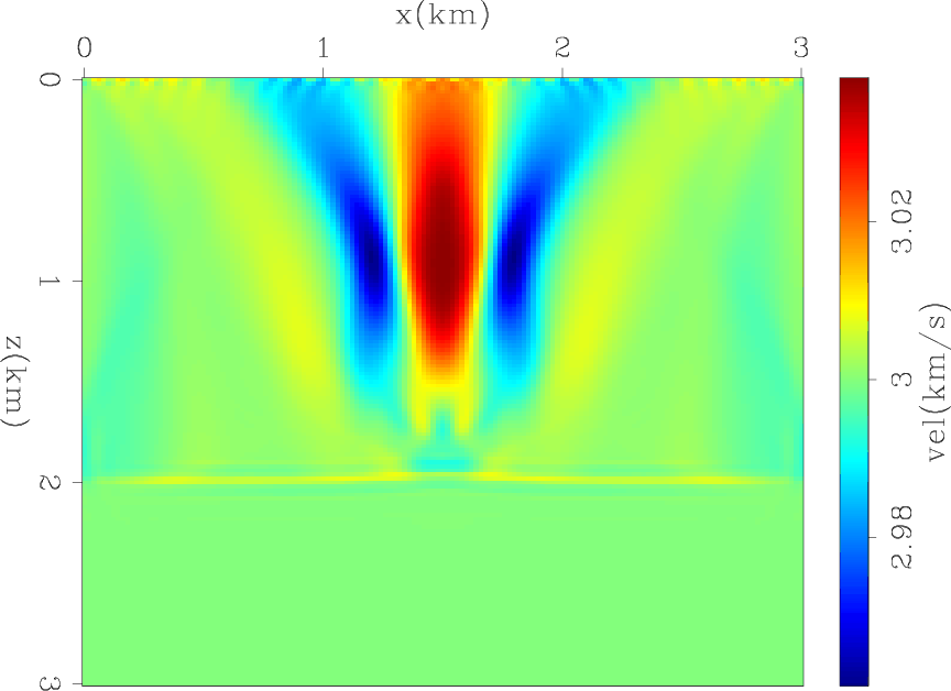
Figure 5. The inverted background of the Gaussian model example with mixing of scales.

gauss-imodelr2
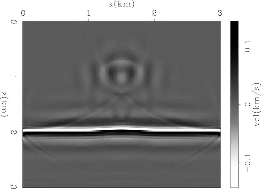
Figure 6. The inverted reflectivity of the Gaussian model example with mixing of scales.

Figures 3 and 4 shows the final background and reflectivity models without scale mixing. The background has a low vertical resolution with relatively strong side-lobes around the anomaly location. The reflectivity model has a low horizontal resolution where the sides of the anomaly are not well illuminated. This lack of resolution in both models is expected due to the limited acquisition.

Figures 5 and 6 shows the final background and reflectivity models with scale mixing. The background has a much better vertical resolution that locates the anomaly at the correct depth. Moreover, the peak amplitude of the anomaly is more than three times stronger compared to Figure 3 while the side-lobes remained at the same strength. The reflectivity model shows substantial improvements in resolution as well. The sides of the anomaly seem to be better illuminated after scale mixing. Although reflectivity is linear with respect to the data, the inverted model seems to benefit from the scale mixing. Therefore, the contribution of the background gradient seem to add to the null space components of the reflectivity model, and vice-versa.

Tomographic full waveform inversion: Practical and computationally feasible approach