|
|
|
|
Two-parameters residual-moveout analysis for wave-equation migration velocity analysis |
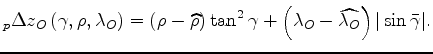
As a quality measurements of the gradient information,
I compute the correlation across the angle axis between
the RMO function that would be computed by picking
the maxima of the coherency spectra
![]() and the RMO function
and the RMO function
![]() computed using the gradient.
computed using the gradient.
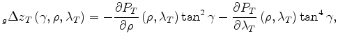
For the ``Taylor'' RMO the reference
RMO function
![]() is computed as follows:
is computed as follows:
 are the coordinates
of the power-spectrum maximum.
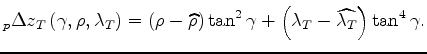
The
RMO function
are the coordinates
of the power-spectrum maximum.
The
RMO function
 computed from the gradient
of the power spectrum
computed from the gradient
of the power spectrum  with the correlation function computed by
 is computed as follows
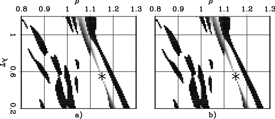
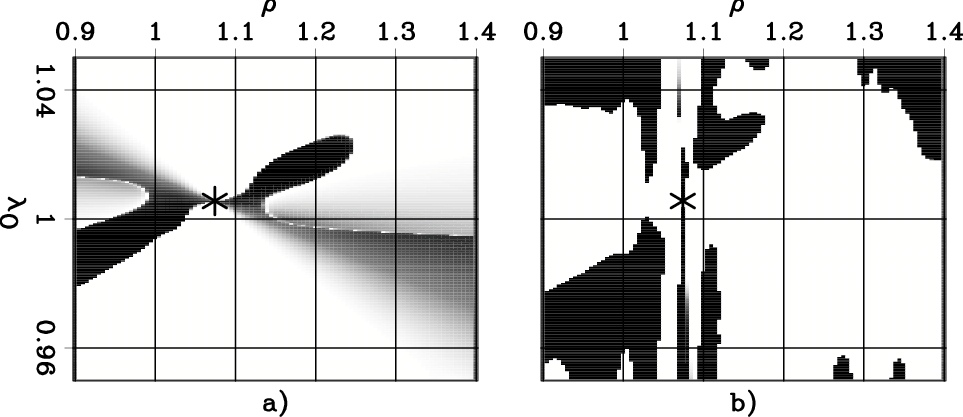
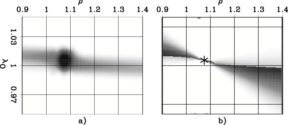
Figure 5
compares the correlation functions  (panel a)
and
(panel a)
and ![]() (panel b)
for the first CIG analyzed (Figure 1a).
The asterisk superimposed onto the plots of the correlation functions
is located at the maximum of the power spectrum
displayed in Figure 2a.
The coordinates
of this maximum are used to evaluate the moveout
(panel b)
for the first CIG analyzed (Figure 1a).
The asterisk superimposed onto the plots of the correlation functions
is located at the maximum of the power spectrum
displayed in Figure 2a.
The coordinates
of this maximum are used to evaluate the moveout
![]() according to equation 4.
Accurate gradient directions correspond to positive correlation
(plotted in white in the figure),
whereas potentially misleading gradient directions
correspond to negative correlation (plotted in black in the figure).
according to equation 4.
Accurate gradient directions correspond to positive correlation
(plotted in white in the figure),
whereas potentially misleading gradient directions
correspond to negative correlation (plotted in black in the figure).
The correlation functions are mostly positive over a wide
range of parameters
,
indicating that a velocity estimation method based on these RMO functions
is likely to have good global convergence properties.
In particular,
the positive correlation functions at
![]() indicates that the gradient computed starting from the
migrated CIG shown in Figure 2a
would be accurate, even if this CIG is far from being flat.
indicates that the gradient computed starting from the
migrated CIG shown in Figure 2a
would be accurate, even if this CIG is far from being flat.
The correlation functions shown in Figure 5 are very similar. Therefore, the global convergence of the velocity estimation would be robust independently of whether the one-parameter or the two-parameter RMO function is used.
|
|---|
|
CorrShift-TP
Figure 5. Correlation functions corresponding to the CIG shown in Figure 1a for: a) the ``Taylor'' two-parameter RMO function (equation 6), and b) the one-parameter RMO function (equation 7). |
|
|
|
|---|
|
CorrShift-OP
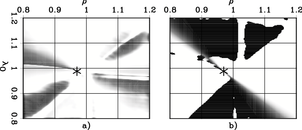
Figure 6. Correlation functions corresponding to the CIG shown in Figure 1a for: a) the ``Orthogonal'' two-parameter RMO function (equation 11), and b) the one-parameter RMO function (equation 12). |
|
|
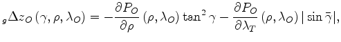
Similar correlation analysis of the RMO function can be performed when
applying the ``Orthogonal'' RMO instead of the ``Taylor'' RMO.
In this case the reference
RMO function
![]() is computed as follows:
is computed as follows:
 are the coordinates
of the corresponding power-spectrum maximum.
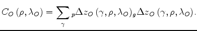
The
RMO function
are the coordinates
of the corresponding power-spectrum maximum.
The
RMO function
 computed from the gradient
of the power spectrum
computed from the gradient
of the power spectrum 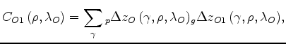 is computed as follows
Figure 6
compares the correlation functions 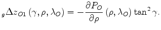 (panel a)
and
(panel a)
and ![]() (panel b)
for the first CIG analyzed (Figure 1a).
The asterisk superimposed onto the plots of the correlation functions
is located at the maximum of the power spectrum
displayed in Figure 2b.
The coordinates
of this maximum are used to evaluate the moveout
(panel b)
for the first CIG analyzed (Figure 1a).
The asterisk superimposed onto the plots of the correlation functions
is located at the maximum of the power spectrum
displayed in Figure 2b.
The coordinates
of this maximum are used to evaluate the moveout
![]() according to equation 9.
As for the previous figure,
accurate gradient directions correspond to positive correlation
(plotted in white in the figure),
whereas potentially misleading gradient directions
correspond to negative correlation (plotted in black in the figure).
according to equation 9.
As for the previous figure,
accurate gradient directions correspond to positive correlation
(plotted in white in the figure),
whereas potentially misleading gradient directions
correspond to negative correlation (plotted in black in the figure).
In this case the correlation functions
shown in Figure 6
are not as similar as in the previous case.
In particular, the black area around
the value
![]() in Figure 6a
indicate that the two-parameter RMO analysis would provide
unreliable gradients.
This problem is related to the diagonal artifacts
visible in the power spectrum shown in
in Figure 2a.
These artifacts are caused by the fact that the second term
in the ``Orthogonal'' RMO function has an extremum
in the middle of the angular range,
in contrast with the other RMO functions that have
an extremum at normal-incidence.
This mid-range extremum causes spurious local maxima of the spectrum
at depths different than the normal incidence depth of the imaged reflector.
These artifacts are much weaker
when I averaged the power spectrum over a thinner depth interval (30 m)
than the one used for computing the function displayed in
Figure 6a.
The new averaging window is of thickness comparable
to the image of the reflector.
Figure 7a
shows the power spectrum obtained with this thinner averaging window,
and Figure 7b
corresponds to the two-parameters correlation function,
which is a substantial improvement with respect to the one
shown in Figure 6a.
in Figure 6a
indicate that the two-parameter RMO analysis would provide
unreliable gradients.
This problem is related to the diagonal artifacts
visible in the power spectrum shown in
in Figure 2a.
These artifacts are caused by the fact that the second term
in the ``Orthogonal'' RMO function has an extremum
in the middle of the angular range,
in contrast with the other RMO functions that have
an extremum at normal-incidence.
This mid-range extremum causes spurious local maxima of the spectrum
at depths different than the normal incidence depth of the imaged reflector.
These artifacts are much weaker
when I averaged the power spectrum over a thinner depth interval (30 m)
than the one used for computing the function displayed in
Figure 6a.
The new averaging window is of thickness comparable
to the image of the reflector.
Figure 7a
shows the power spectrum obtained with this thinner averaging window,
and Figure 7b
corresponds to the two-parameters correlation function,
which is a substantial improvement with respect to the one
shown in Figure 6a.
|
|---|
|
CorrShift-OP-narrow
Figure 7. Panel a): Two-parameter stack-power spectra resulting from RMO analysis of the CIG shown in Figure 1a obtained using a thinner averaging window (30 m) than the one used to compute the spectrum shown in Figure 2b. Panel b): Correlation function for the ``Orthogonal'' two-parameter RMO function obtained using the thinner averaging window. |
|
|

|
|---|
|
CorrShift-TP-aniso
Figure 8. Correlation functions corresponding to the CIG shown in Figure 3a for: a) the ``Taylor'' two-parameter RMO function (equation 6), and b) the one-parameter RMO function (equation 7). |
|
|
|
|---|
|
CorrShift-OP-aniso
Figure 9. Correlation functions corresponding to the CIG shown in Figure 3a for: a) the ``Orthogonal'' two-parameter RMO function (equation 11), and b) the one-parameter RMO function (equation 12). |
|
|
|
|
|
|
Two-parameters residual-moveout analysis for wave-equation migration velocity analysis |