 |
 |
 |
 | Preconditioned least-squares reverse-time migration using random phase encoding |  |
![[pdf]](icons/pdf.png) |
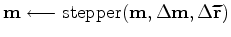
Next: Synthetic Examples
Up: Method
Previous: Least-squares RTM
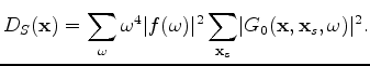
For any linear operator  , the Hessian matrix is computed as follows:
 |
(13) |
where  and
and 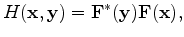 are model coordinates. There are several ways to utilize the Hessian matrix in the inversion process, but I will focus on using its diagonal as a preconditioner to the gradient:
 |
(14) |
where
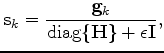 is gradient at the
 iteration,
 is the preconditioned search direction,
  is an identity operator, and
  is a constant used to stabilize the division. For the modeling operator, the diagonal of the Hessian matrix can be written as follows:
 |
(15) |
Unlike with forward and adjoint modeling operators, the computations must be done on each source-receiver pair separately. As with LSRTM, the expense of this operation can be reduced by encoding the source or receiver side, or both sides. I first define a receiver-side encoding function 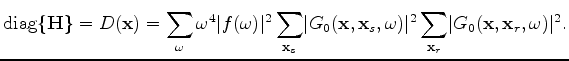 as follows:
 |
(16) |
where 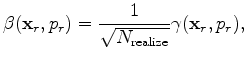 is the realization index, and the other variables are the same as in the encoding function
  . I now define an encoded receiver wavefield:
 |
(17) |
This encoding results in the receiver-side blended function
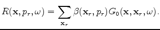 , which can be written as follows:
 |
(18) |
The cost of one realization of the function
is equivalent to an unblended migration of all the shots. Additionally, the source side can also be blended:
 |
(19) |
The cost of one realization of the function
 is equivalent to migrating one shot only. However, the additional blending results in more crosstalk. Hence, the function
requires more realizations to reduce the crosstalk artifacts than does the function
.
is equivalent to migrating one shot only. However, the additional blending results in more crosstalk. Hence, the function
requires more realizations to reduce the crosstalk artifacts than does the function
.
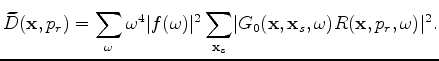
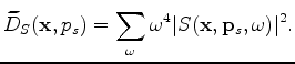
Although the cost of computing the function  can be reduced with blending, additional propagation(s) are still required to compute the receiver side. Therefore, preconditioning with the source intensity function
 can be done by ignoring the receiver side of the Hessian matrix. The source intensity function can be written as follows:
 |
(20) |
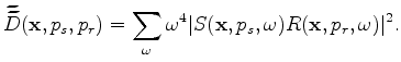
The previous formulation computes the exact source function in one iteration of LSRTM. However, if the inversion is done with the blended operator, the source intensity function can be computed using the blended source wavefield as follows:
 |
(21) |
By comparing equation (21) to equation (19), we can see that ignoring the receiver side in the Hessian matrix can be physically interpreted as having receivers everywhere in the subsurface. As a result, the source intensity function overestimates the Hessian matrix. Therefore, I propose a better approximation to the Hessian matrix by using the blended source wavefiled to approximate the receiver-side. This source-based Hessian can be written as follows:
 |
(22) |
The function
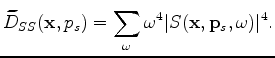 approximates the receiver wavefield by the source wavefield. Physically, this assumes that the receivers exist at the same location as the sources. This is a better approximation than the original source intensity function, especially for the fixed-spread geometry. This formulation requires no additional propagation if the source side is blended. However, there are two sources of error in equation (22). First, the receiver spacing could be different than the source spacing, even if their spreads cover the same area. Second, the receiver side should have a different encoding function than the source side. These errors will prevent the source-based Hessian from approaching the true Hessian matrix, regardless of the number of realizations.
|
|
|
|
| Preconditioned least-squares reverse-time migration using random phase encoding | |
|
Next: Synthetic Examples
Up: Method
Previous: Least-squares RTM
2011-09-13