|
|
|
|
Preconditioned least-squares reverse-time migration using random phase encoding |
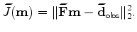
 is the surface data and
 The
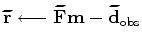
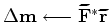
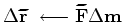
iterate {


}
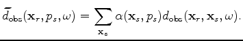
There are several encoding functions that can be used in LSRTM (Godwin and Sava, 2011; Perrone and Sava, 2009). However, a single-sample random phase function gives the best convergence results (Romero et al., 2000; Krebs et al., 2009). This encoding function results in crosstalk artifacts in the estimated models. These artifacts are reduced by averaging several realizations of the encoding function. The source-side encoding function ![]() is defined as follows (Tang, 2009):
is defined as follows (Tang, 2009):
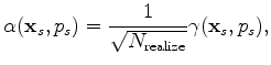 is the realization index,
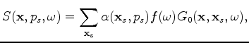 is the blended source wavefield. Due to the linearity of the wave equation, this wavefield can be simply computed by simultaneously injecting the source functions at different locations after multiplying by the proper weight. Once
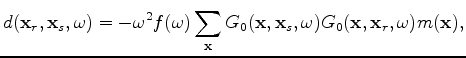
is computed, the blended forward modeling operator can defined as follows:
is the blended source wavefield. Due to the linearity of the wave equation, this wavefield can be simply computed by simultaneously injecting the source functions at different locations after multiplying by the proper weight. Once
is computed, the blended forward modeling operator can defined as follows:
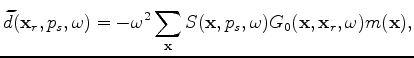 is used to indicate blending. The blended forward modeling operator
		 iterate {


}
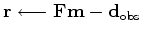
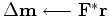
There are two changes in the minimization scheme of the blended objective function compared to the conventional one. First, the computation of the residual is moved inside the loop, because the encoding function changes in each iteration. This change adds the cost of a forward modeling operator to each iteration. Second, the stepper algorithm can only be steepest-descent if the step size is determined with linear optimization. Otherwise, a non-linear conjugate gradient can be performed, requiring a line search in each iteration. In this paper I present only the result of using steepest-descent stepper, because the iteration cost is consistent.
|
|
|
|
Preconditioned least-squares reverse-time migration using random phase encoding |