Preconditioned least-squares reverse-time migration using random phase encoding

Synthetic Examples

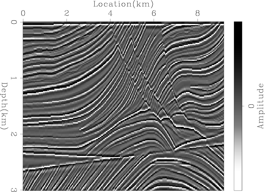
A decimated Marmousi model is used for the synthetic examples. The sampling for both spatial axes is 20 m. A Ricker wavelet with a fundamental frequency of 15 Hz and temporal sampling of 1.5 ms is used to model the data. The receiver spacing is 20 m, and the source spacing is 100 m. Born modeling with a time-domain finite-difference propagator was used in both the observed and the calculated data.

marmousi,marmousi-smooth
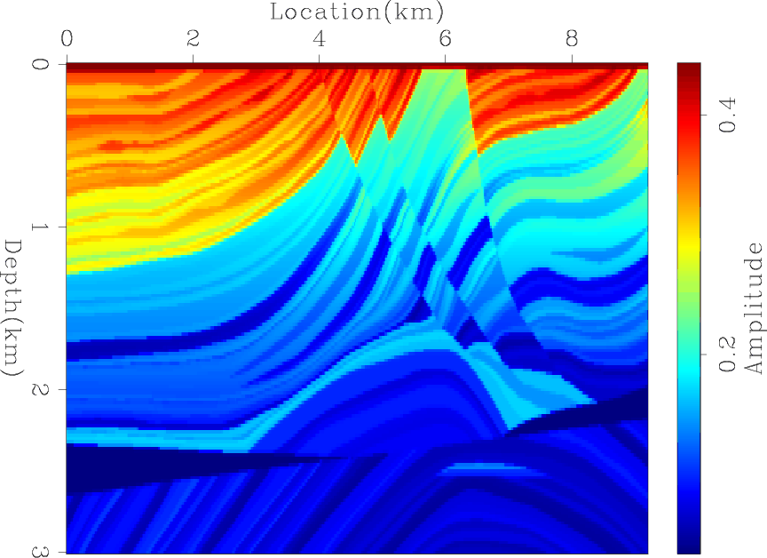
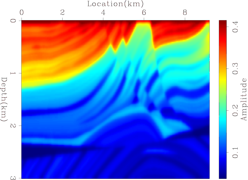
Figure 1. (a) Marmousi slowness squared and (b) the background model.

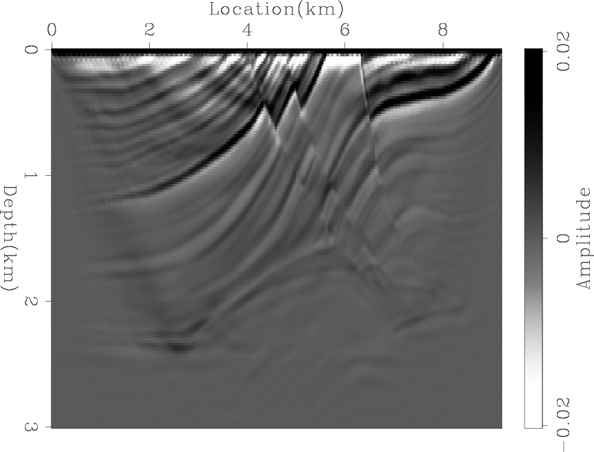
Figures 1(a) and 1(b) show the Marmousi slowness squared and the background model, respectively. The reflectivity model, obtained by subtracting the Marmousi slowness squared from the background model, is shown in Figure 2.

marmousi-refl
Figure 2. The Marmousi reflectivity model.

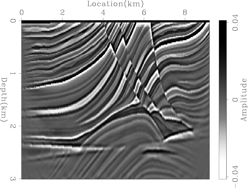
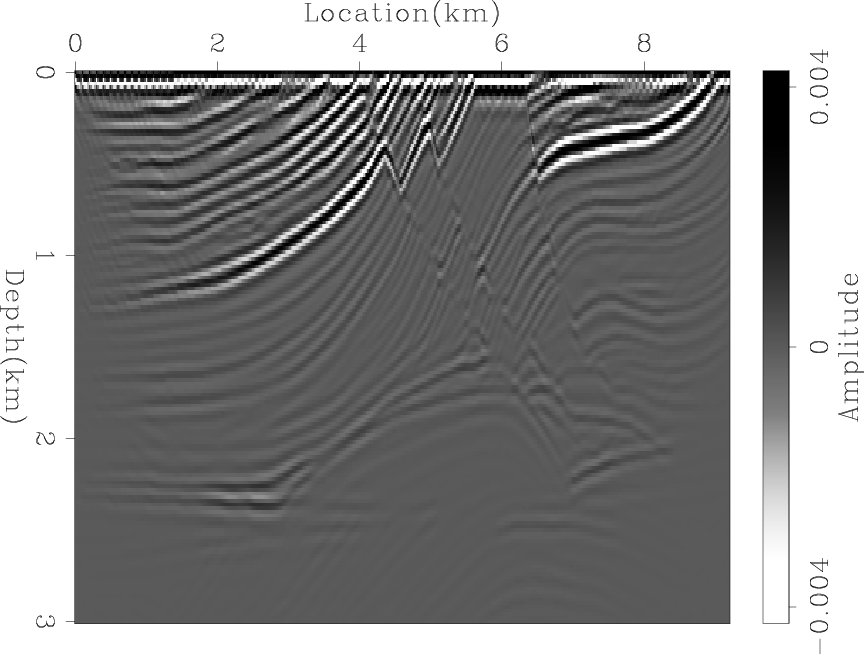
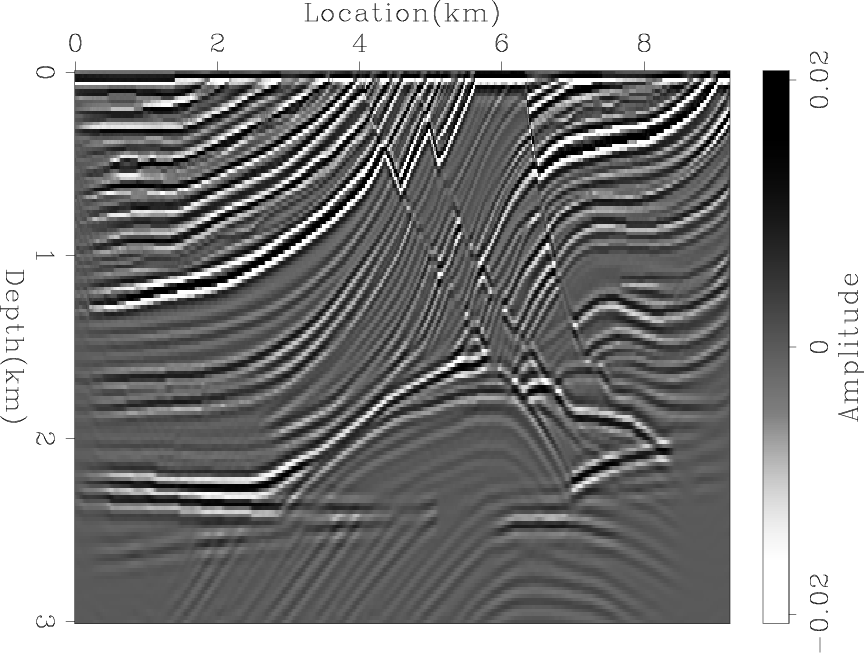
First, I ran a conventional LSRTM without any preconditioning for 50 iterations. The result of the fifth iteration is shown in Figure 3(a). This result is dominated by low-frequency noise as well as strong imbalance in amplitudes of the model. Next, I repeated the experiment, this time blending the sources. Figure 3(b) shows the result after 310 iterations, which is equivalent in cost to five iterations of unblended LSRTM. By comparing Figures 3(a) and 3(b), we see the blended LSRTM gives much better results.

marmousi-lsrtmcd,marmousi-lsrtmb
Figure 3. (a) Conventional LSRTM after 5 iterations and (b) blended LSRTM after 310 iterations.

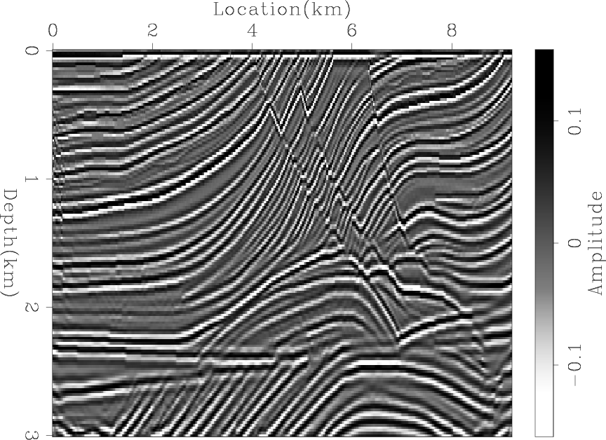
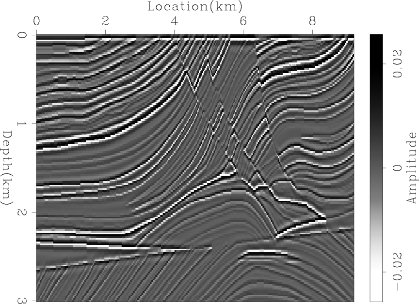
In order to determine whether the difference between the two results is only caused by the low frequency noise, I applied a low-cut filter to both results, as shown in Figures 4(a) and 4(b). Next, I further processed the results to remove the amplitude imbalance by applying an AGC, as shown in Figures 5(a) and 5(b). For comparison, Figures 6(a) and 6(b) show the true reflectivity model after applying the same processing steps. We can see that the blended LSRTM gives sharper and more accurate images even after processing.

marmousi-lsrtmcd-bp,marmousi-lsrtmb-bp
Figure 4. The result of applying a low-cut filter to Figures 3(a) and 3(b).

marmousi-lsrtmcd-agc,marmousi-lsrtmb-agc
Figure 5. The result of applying an AGC to Figures 4(a) and 4(b).

marmousi-refl-bp,marmousi-refl-agc
Figure 6. The result of applying (a) a low-cut filter and (b) an AGC to Figure 2.

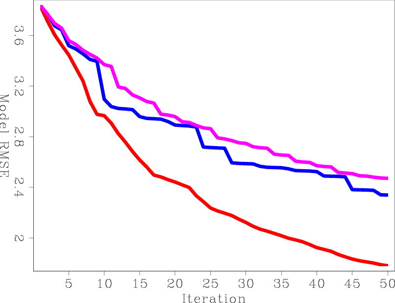
For a more accurate measure of error, I computed the RMS error between the true reflectivity model and the result of each iteration before processing. Figure 7(a) shows three curves: the unblended LSRTM using steepest-descent stepper (LSRTM-SD), the unblended LSRTM using conjugate-direction stepper (LSRTM-CD), and blended LSRTM using steepest-descent stepper (B-LSRTM). It is interesting to see that the blended LSRTM is converging at a similar rate to the unblended LSRTM with the steepest-descent stepper, although their costs are very different. This seems to indicate that while suppressing the crosstalk, the blended LSRTM is also inverting the operator without much loss of efficiency. The only advantage for unblended LSRTM seems to result from having a better stepper.

lsrtm-obj,lsrtm-obj-cost
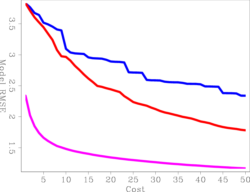
Figure 7. The model RMS error versus (a) iteration and (b) migration cost. LSRTM-SD is blue, SLRTM-CD is red, and B-LSRTM is purple.

Figure 7(b) shows the RMS error curves as a function of cost. The cost unit is equivalent to a conventional RTM of all the shots. This Figure clearly shows that for the same cost, the B-LSRTM gives much better results than the conventional LSRTM regardless of the stepper algorithm.

lsrtm-obj-agc,lsrtm-obj-agc-cost
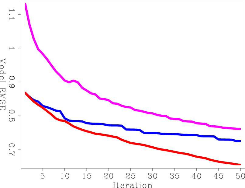
Figure 8. The same as Figures 7(a) and 7(b) but after processing the inversion results with a low-cut filter and AGC. LSRTM-SD is blue, SLRTM-CD is red, and B-LSRTM is purple.

Figure 8(a) is the same as Figure 7(a), but after processing the inversion results. The B-LSRTM seems to have a much larger initial error because the crosstalk artifacts, which are high frequency, are amplified by applying a low-cut filter. However, by comparing the results at the same cost, as shown in Figure 8(b), the B-LSRTM is still superior to the other unblended LSRTM inversions.

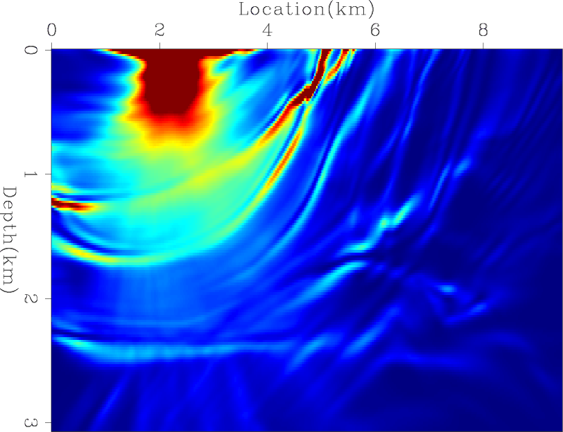
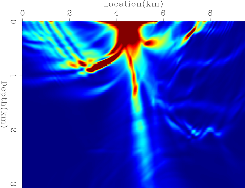
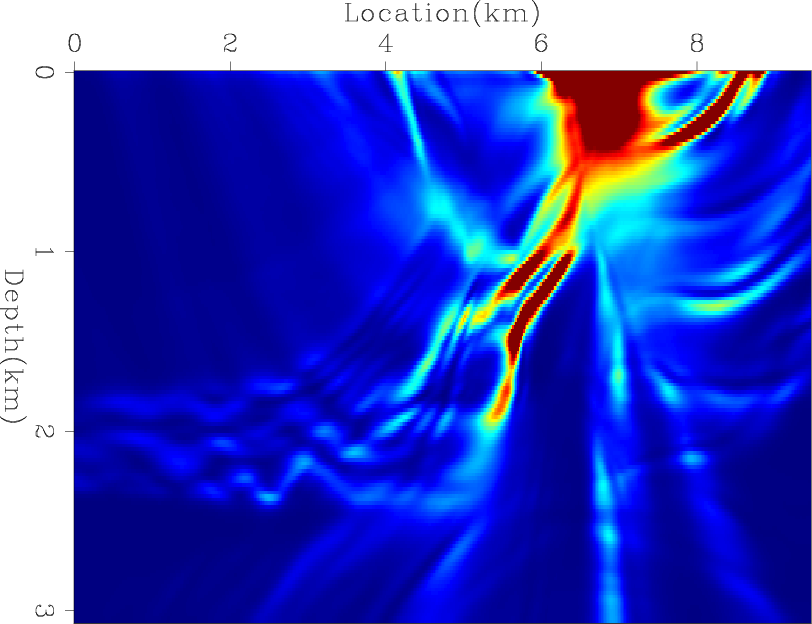
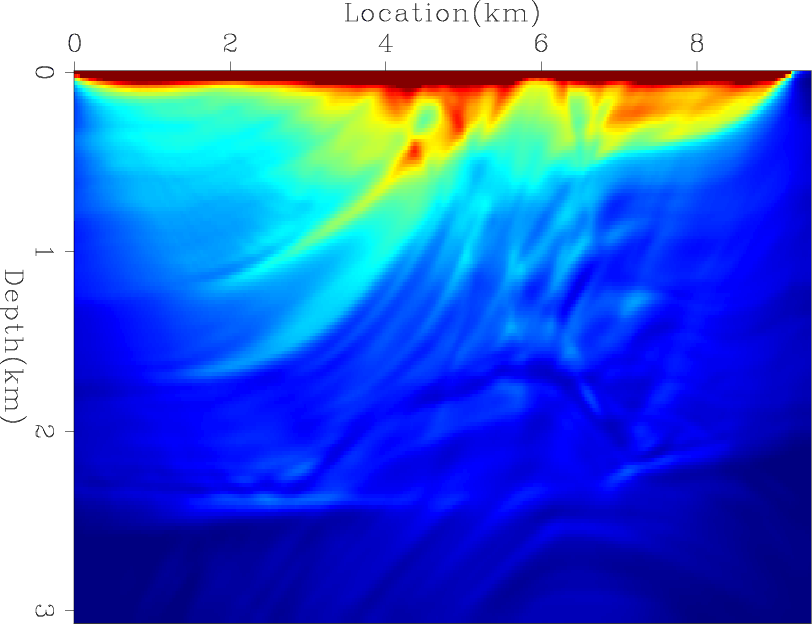
hess1,hess2,hess3,hess
Figure 9. (a), (b), and (c) show the contributions of three different shots and (d) shows the total diagonal of the Hessian matrix.

hess-obj,hess-obj-cost
Figure 10. The model RMS error of (a) every iterations/realization and (b) every migration cost. HRB is blue, HSRB is red, SISB is green, SHSB and is purple.

Next, I computed the exact diagonal of the Hessian matrix. Figures 9(a), 9(b), and 9(c) shows the contribution from three different shots, and Figure 9(d) shows the total diagonal of the Hessian matrix. I then tested the convergence rates of four preconditioners: the Hessian matrix with receiver-side blending (HRB), the Hessian matrix with source- and receiver-side blending (HSRB), the source intensity function with source-side blending (SISB), and the source-based Hessian with source-side blending (SHSB).

hess-hrb,hess-hsrb,hess-sisb,hess-shsb
Figure 11. The results after 50 migrations equivalent cost of (a) HRB, (b) HSRB, (c) SISB, and (d) SHSB.

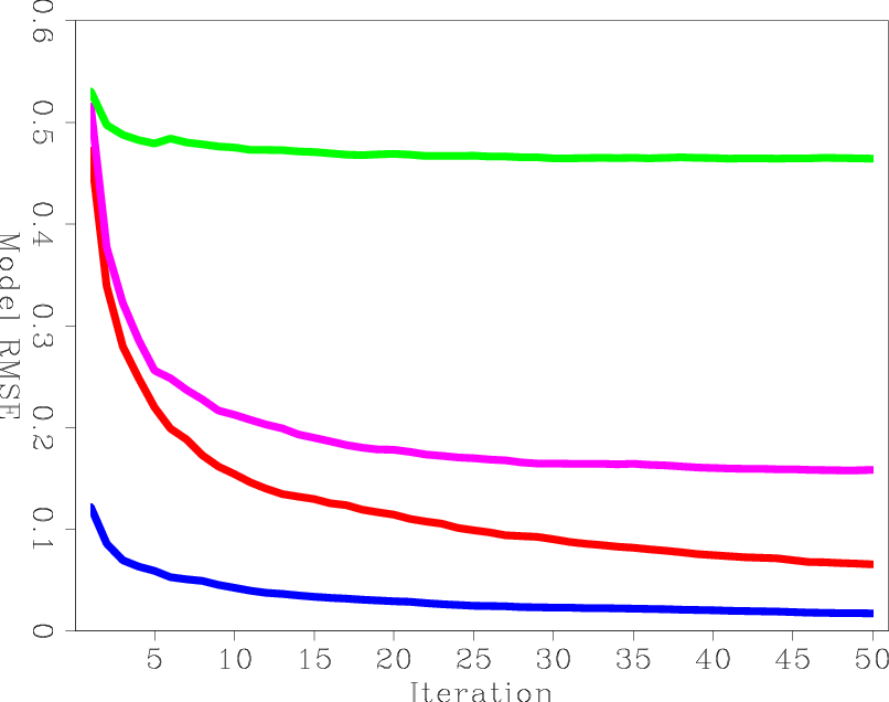
Figures 10(a) and 10(b) show the RMS error of each preconditioner compared to the exact Hessian diagonal versus iteration and versus cost, respectively. Both HRB and HSRB approach the true Hessian diagonal, but encoding both sides gives a faster convergence rate per cost. The SISB converges the fastest, but it converges to a solution with a large error. On the other hand, SHSB converges to a much better solution and at a similar rate to SISB. The preconditioners after 50 migrations equivalent cost are shown in Figures 11(a), 11(b), 11(c), and 11(d).

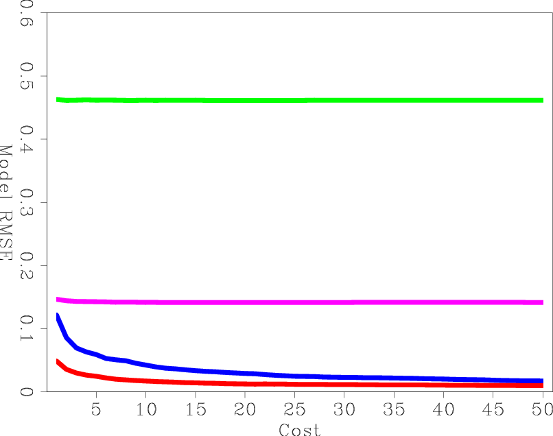
lsrtm-objp,lsrtm-objp-cost
Figure 12. The model RMS error versus (a) iteration and (b) migration cost. No preconditioning is blue, HRSB is green, SISB is red, SHSB and is purple.

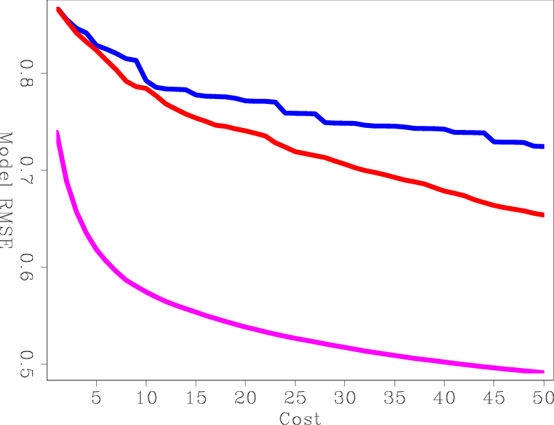
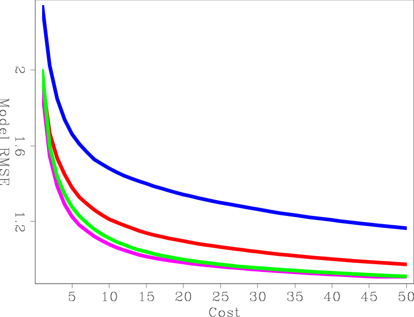
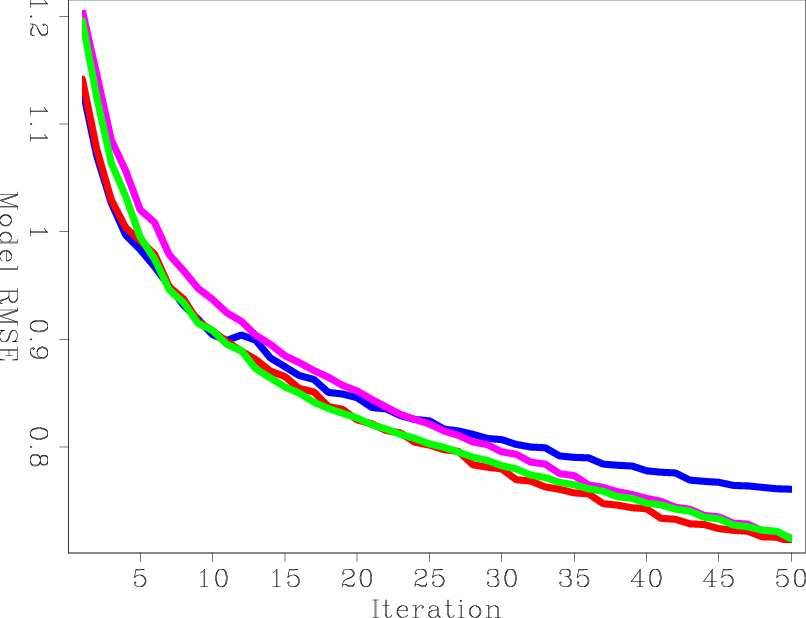
Finally, I ran three LSRTM inversions using HRSB, SISB, and SHSB as preconditioners and compared them to the unpreconditioned B-LSRTM. Figure 12(a) shows the model RMS error of the four curves as a function of iteration. The three preconditioned curves seems to converge at a simiar rate per iteration. However, the convergence rates per cost are different, as shown in Figure 12(b). Although SHSB had larger error in estimating the Hessian matrix, it resulted in the best convergence rate for LSRTM due to its cheaper cost. The second-best method was HRSB.

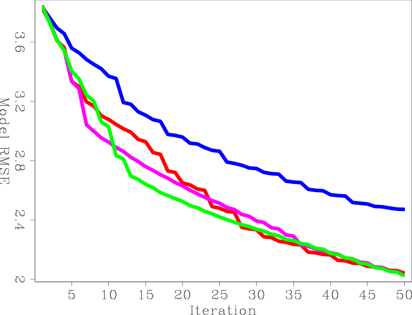
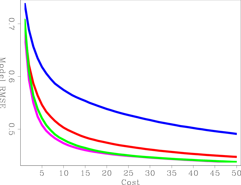
As with the previous LSRTM, I processed the results of preconditioned LSRTM and compared it to the processed, true reflectivity. Figures 13(a) and 13(b) show the model RMS error versus iteration and cost, respectively. Processing the models did not change the order of the curves, but, as expected, it reduced the difference between them in the early iterations.

lsrtm-objp-agc,lsrtm-objp-agc-cost
Figure 13. The same as Figures 12(a) and 12(b) but after processing the inversion results with a low-cut filter and AGC. No preconditioning is blue, HRSB is green, SISB is red, SHSB and is purple.

Preconditioned least-squares reverse-time migration using random phase encoding