A new algorithm for bidirectional deconvolution

2D synthetic data

After applying deconvolution on the simple 1D case, we test the Zhang and Claerbout (2010) method and our new method on more complicated 2D synthetic data. Figure 9(a) shows the starting reflectivity model. Figure 9(b) shows the data generated by convolving the reflectivity model with the zero-phase wavelet in the previous section. All traces use the same wavelet when generating the data, and all traces share the same wavelet when we are doing the deconvolution.

syn3,data3
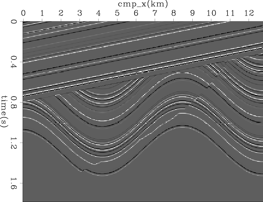
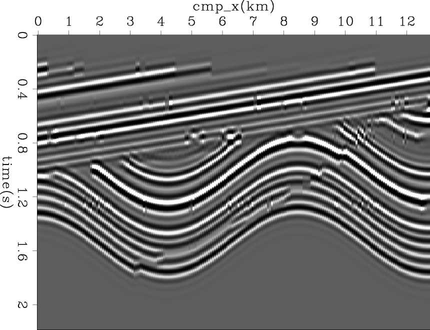
Figure 9. (a) The 2D synthetic reflectivity model; (b) the synthetic data generated using the zero-phase wavelet.

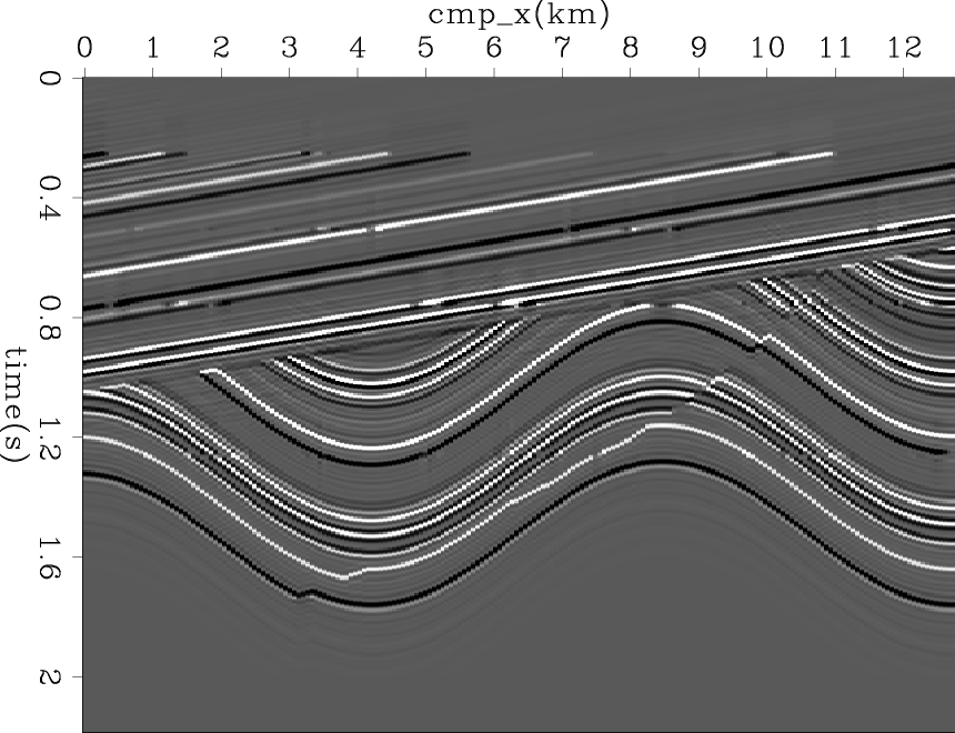
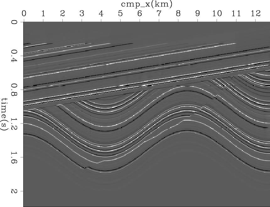
Figures 10(a) and 10(b) show the bidirectional deconvolution using our method and the older method. Both methods retrieve the sparse reflectivity model and compress the wavelet into a spike, but the deconvolution model produced by the previous method is more spiky than ours, just as in the previous section, because of the wavelet we use.

We also compare the computational costs of these two methods. To deal with this synthetic data, we use 2 linear iterations and 280 non-linear iterations to reach convergence, whereas Zhang and Claerbout (2010) used 100 linear iterations and 20 non-linear iterations, a total of 2000 iterations. In fact, our code is almost 6 times faster than the previous method.

mod3new,mod3old
Figure 10. Given the 2D synthetic data in Figure 9(b), (a) reflectivity model retrieved using our method; (b) reflectivity model retrieved using the previous method.

A new algorithm for bidirectional deconvolution