A new algorithm for bidirectional deconvolution

Single wavelet

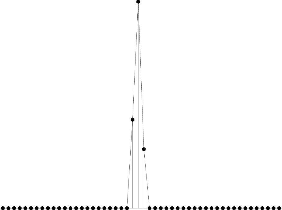
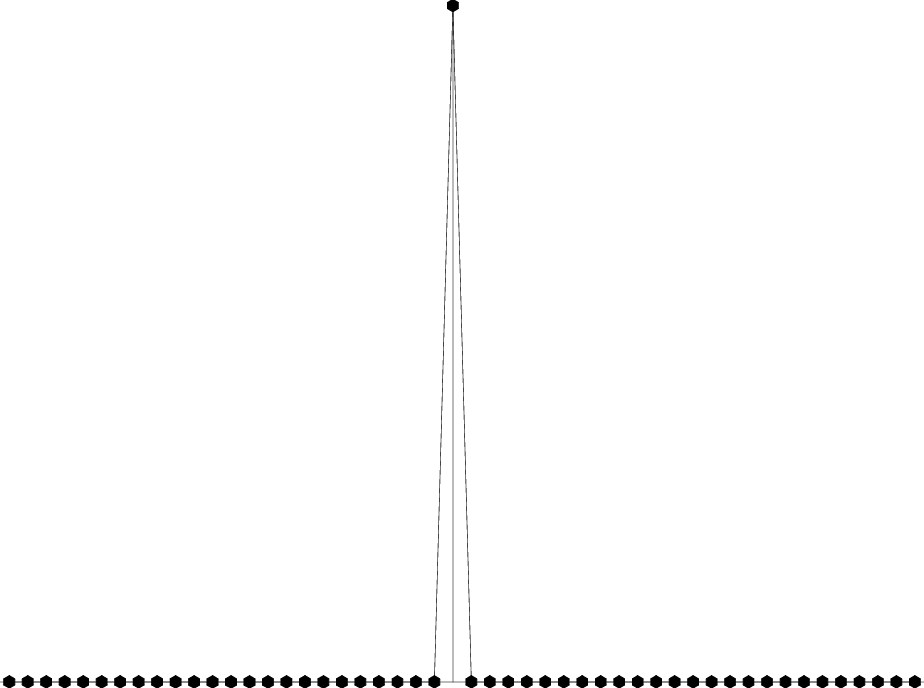
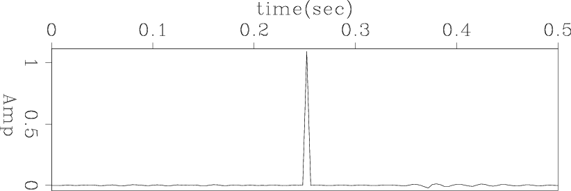
The first data example is the simplest mixed-phase wavelet, which only has three points [3,7,2]. We use it to verify the ability of our method to deal with the mixed-phase wavelet. The input data and its bidirectional result are shown in Figures 1 and 2. In this case, our new method is able to compress the simple mixed phase wavelet into a spike.

data1 Figure 1. The three data points [3,7,2].

mod1 Figure 2. The result of our deconvolution method.

To illustrate the capabilities and limitations of our new method, we analyze the results obtained by inverting the zero-phase wavelet. This wavelet is created by convolving the minimum-phase with its own time-reversed wavelet.

Figures 3(a) and 3(b) show the filters estimated by our method. Figures 3(c) and 3(d) show the filters inverted by the previous method of bidirectional deconvolution. Here we time-reverse the anti-causal filter $b^r$ into a causal filter $b$ for easier comparison. Ideally, filter $a$ and filter $b$ should be identical, because the zero-phase wavelet is symmetric, with its minimum-phase part the same as its maximum-phase part, but time-reversed. The results of our method perfectly satisfy the theory, which shows the extreme similarity between filter $a$ and filter $b$ . When we invert the filters, the update direction is the same for both filters, because the searching gradients are equal. However, using the method from Zhang and Claerbout (2010) yields a filter $a$ that is quite different from filter $b$ , because they are inverted separately.

filt2anew,filt2bnew,filt2aold,filt2bold
Figure 3. For zero-phase wavelet inversion, (a) filter $a$ estimated by our method; (b) filter $b$ estimated by our method; (c) filter $a$ estimated by the previous method; (d) filter $b$ estimated by the previous method.

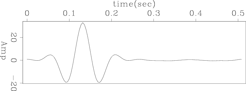
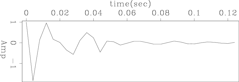
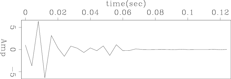
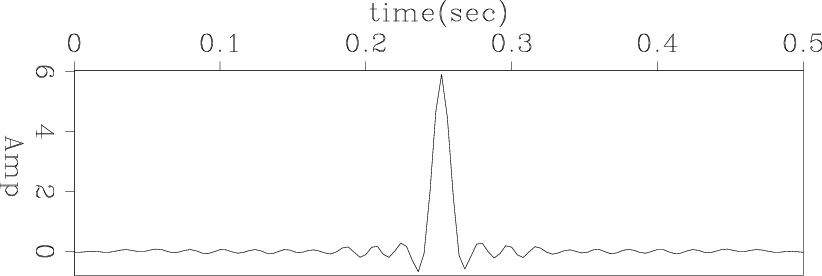
Figures 4, 5 and 6 show the zero-phase wavelet and its bidirectional deconvolution, using our new algorithm and the method of Zhang and Claerbout (2010). The results show that the wavelet is almost compressed into a spike by our method, but it is not as spiky as the result of the previous method. One possible reason may be the nature of the non-linear problem. There may be multiple minima in this problem, and due to our additional condition that filter $a$ and filter $b$ should be the same in this case, we find a different minimum, which leads to a different result.

Thus a good starting guess may help us to get a better result. Or perhaps the preconditioning can also make the solution fast converge to the global minima by utilizing prior information.

data2 Figure 4. Zero-phase wavelet.

mod2new Figure 5. Deconvolution result by our method.

mod2old Figure 6. Deconvolution result by the previous method.

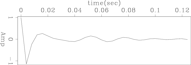
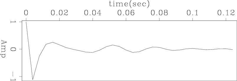
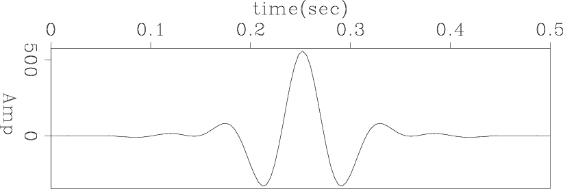
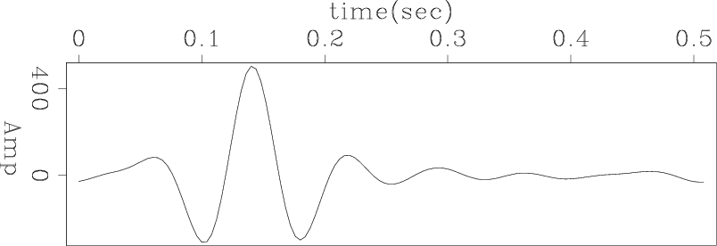
Figures 7 and 8 show the wavelet estimated by our method and the previous method. We notice that both of the wavelets approximate the input zero-phase wavelet, which is shown in Figure 4. However our estimated wavelet looks more symmetric and cleaner with less side lopes than the one estimated by the previous method. The reason is that our estimated filters are identical, which make the causal part and anti-causal part of the inverted wavelet the same.

wavelet2new Figure 7. Shot wavelet estimated by our method

wavelet2old Figure 8. Shot wavelet estimated by the previous method

A new algorithm for bidirectional deconvolution