A new algorithm for bidirectional deconvolution

2D field data

The field data we use in this example is a common-offest section of marine field data. Figure 11 shows the input data. Figures 12(a) and 12(b) show the bidirectional deconvolution using our method and the previous method. Both perform well to retrieve the sparse reflectivity in this field data.

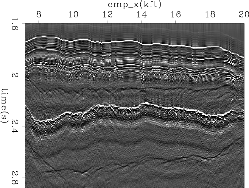
data4
Figure 11. Input Common Offset data.

mod4new,mod4old
Figure 12. Given the common offset data in Figure 11, (a) reflectivity model retrieved using our method; (b) reflectivity model retrieved using the previous method.

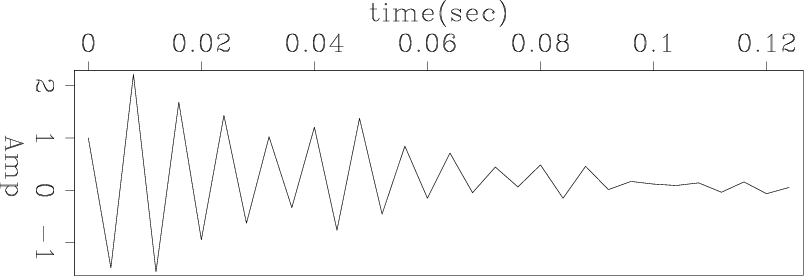
The filters estimated by our method are shown in Figures 14(a), and 14(b), and the filters estimated by the previous method are plotted in Figures 14(c) and 14(d). Because the wavelet we aim to invert is not symmetric, filter $a$ and filter $b$ are not equal. However, the strong events look like a double ghost (white, black,white), which approximates a symmetric wavelet. Thus we would like our filters to resemble each other. From the result, we notice that our filters satisfy these expectation.

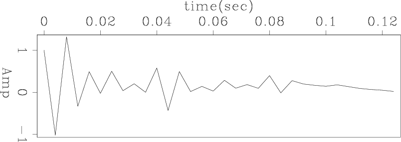
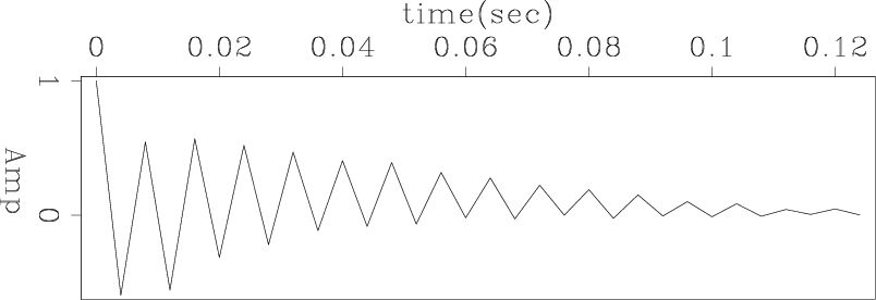
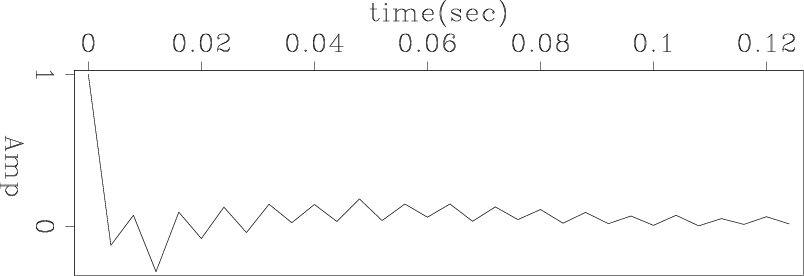
Figures 13(a) and 13(b) show the estimated shot waveform. The data sampling is 4ms. We notice that both of our method estimate the bubbles and the double ghost. However, our inverted waveform is more like a double ghost, which can be noticed in the data. The reason is that our filters more resemble each other than the ones estimated by the previous method.

wavelet4new,wavelet4old
Figure 13. For 2D synthetic data, (a) shot wavelet estimated by our method; (b) shot wavelet estimated by the previous method.

filt4anew,filt4bnew,filt4aold,filt4bold
Figure 14. Given the common offset data in Figure 11, (a) filter $a$ estimated by our method; (b) filter $b$ estimated by our method; (c) filter $a$ estimated by the previous method; (d) filter $b$ estimated by the previous method.

Our method requires 2 linear iterations and 100 non-linear iterations, or only 200 iterations in total. Zhang and Claerbout (2010) used 100 iterations and 8 non-linear iterations, or 800 iterations in total. Therefore, our method is four times faster, which is a large reduction in computational cost.

A new algorithm for bidirectional deconvolution