The stretch factor in time

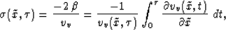
In this appendix, we derive $\sigma$, given by equation 6, in the $(x-\tau)$-domain. Using such an equation can avoid the process of mapping $\sigma$ from depth to time and back. The vertical two-way traveltime, $\tau$, is written as  

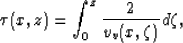$$\tau(x,z) = \int_0^z \frac{2}{v_v(x,\zeta)} d\zeta,$$ (29)

where z corresponds to depth. Similarly,  

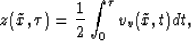$$z(\tilde{x},\tau) = \frac{1}{2} \int_0^{\tau} v_v(\tilde{x},t) dt,$$ (30)

where $\tilde{x}$ corresponds to the new coordinate system.

Using the chain rule,  

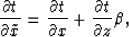$$\frac{\partial t}{\partial \tilde{x}} = \frac{\partial t}{\partial x} + \frac{\partial t}{\partial z} \beta,$$ (31)

where $\beta$ extracted from equation (30) is given by  

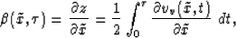$$\beta (\tilde{x},\tau)= \frac{\partial z}{\partial \tilde{x}... ...u} \frac{\partial v_v(\tilde{x},t)}{\partial \tilde{x}}\,\, dt,$$ (32)

the partial derivative in $\tau$ is  

$$\frac{\partial t}{\partial \tau} = \frac{v_v}{2} \frac{\partial t}{\partial z}.$$ (33)

Therefore, the transformation from ($\tilde{x}$, $\tau$) to (x, z) is governed by the following Jacobian matrix in 2-D:

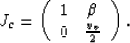$$J_c = \left(\begin{array} {cc} 1& \beta \ 0& \frac{v_v}{2}\ \end{array}\right).$$ (34)

The inverse of J_c is

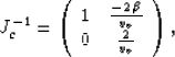$$J_c^{-1} = \left(\begin{array} {cc} 1& {\frac{-2\,\beta }{{v_v}}} \ 0& {\frac{2}{{v_v}}}\ \end{array}\right),$$ (35)

which should equal the Jacobian matrix for the transformation from (x, z) to ($\tilde{x}$, $\tau$), given by

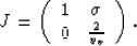$$J = \left(\begin{array} {cc} 1& \sigma\ 0& \frac{2}{v_v}\ \end{array}\right).$$ (36)

As a result,

$$\sigma(\tilde{x},\tau) = \frac{-2\,\beta }{{v_v}} = \frac{... ...u} \frac{\partial v_v(\tilde{x},t)}{\partial \tilde{x}}\,\, dt,$$

which is a convenient equation, since we want to keep all fields, including velocity, in $\tilde{x}-\tau$ coordinates.

B