


Next: Fourier approach
Up: Fomel: Spectral velocity continuation
Previous: Introduction
The post-stack velocity continuation process is governed by a partial
differential equation in the domain, composed by the seismic image
coordinates (midpoint x and vertical time t) and the additional
velocity coordinate v. Neglecting some amplitude-correcting terms
Fomel (1996), the equation takes the form
Claerbout (1986b)
| 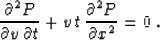 |
(1) |
Equation (1) is linear and belongs to the hyperbolic type. It
describes a wave-type process with the velocity v acting as a
``time-like'' variable. Each constant-v slice of the function
P(x,t,v) corresponds to an image with the corresponding constant
velocity. The necessary boundary and initial conditions are
|  |
(2) |
where v0 is the starting velocity, T=0 for continuation to a
smaller velocity and T is the largest time on the image (completely
attenuated reflection energy) for continuation to a larger velocity.
The first case corresponds to ``modeling''; the latter case, to
seismic migration.
Mathematically, equations (1) and (2) define a
Goursat-type problem Courant (1962). Its analytical solution can be
constructed by a variation of the Riemann method in the form of an
integral operator Fomel (1994, 1996):
|  |
(3) |
where 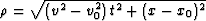 , m=1 in the 2-D
case, and m=2 in the 3-D case. In the case of continuation from zero
velocity v0=0, operator (3) is equivalent (up to the
amplitude weighting) to conventional Kirchoff time migration
Schneider (1978). Similarly, in the frequency-wavenumber
domain, velocity continuation takes the form
, m=1 in the 2-D
case, and m=2 in the 3-D case. In the case of continuation from zero
velocity v0=0, operator (3) is equivalent (up to the
amplitude weighting) to conventional Kirchoff time migration
Schneider (1978). Similarly, in the frequency-wavenumber
domain, velocity continuation takes the form
| 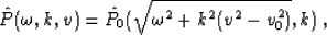 |
(4) |
which is equivalent (up to scaling coefficients) to Stolt migration
Stolt (1985), regarded as the most efficient migration
method.
If our task is to create many constant-velocity slices, there are
other ways to construct the solution of problem (1-2).
Two alternative spectral approaches are discussed in the next two
sections.
Next: Fourier approach
Up: Fomel: Spectral velocity continuation
Previous: Introduction
Stanford Exploration Project
5/1/2000