Next: FROM KINEMATICS TO DYNAMICS
Up: KINEMATICS OF VELOCITY CONTINUATION
Previous: Kinematics of Residual NMO
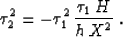
The partial differential equation for kinematic residual DMO is the
third term in (1):
|  |
(30) |
It is more convenient to consider the residual dip-moveout process
coupled with residual normal moveout. Etgen
1990 describes this procedure as the cascade of
inverse DMO with the initial velocity v0, residual NMO, and DMO
with the updated velocity v1. The kinematic equation for residual
NMO+DMO is the sum of the two terms in (1):
|  |
(31) |
If the boundary data for equation (31) are on a
common-offset gather, it is appropriate to rewrite this equation
purely in terms of the midpoint derivative  , eliminating the offset-derivative term
  . The resultant expression, derived in
Appendix A, has the form
. The resultant expression, derived in
Appendix A, has the form
| 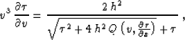 |
(32) |
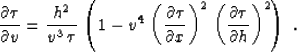
where
|  |
(33) |
The direct solution of equation (32) is nontrivial. A simpler
way to obtain this solution is to decompose residual NMO+DMO into
three steps and to evaluate their contributions separately. Let the
initial data be the zero-offset reflection event  . The
first step of the residual NMO+DMO is the inverse DMO operator. One
can evaluate the effect of this operator by means of the offset
continuation concept Fomel (1995). According to this
concept, each point of the input traveltime curve travels with the change of the offset from zero to h along a special
trajectory, which I call a time ray. Time rays are parabolic
curves of the form
. The
first step of the residual NMO+DMO is the inverse DMO operator. One
can evaluate the effect of this operator by means of the offset
continuation concept Fomel (1995). According to this
concept, each point of the input traveltime curve travels with the change of the offset from zero to h along a special
trajectory, which I call a time ray. Time rays are parabolic
curves of the form
|  |
(34) |
with the final points constrained by the equation
|  |
(35) |
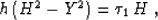
The second step of the cumulative residual NMO+DMO process is the
residual normal moveout. According to equation (23), residual
NMO is a one-trace operation transforming the traveltime  to
to
 as follows:
|  |
(36) |
where
|  |
(37) |
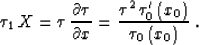
The third step is dip moveout corresponding to the new velocity
v1. DMO is the offset continuation from h to zero
offset along the redefined time rays Fomel (1995)
|  |
(38) |
where  , and
, and  .
The end points of the time rays (38) are defined by the
equation
.
The end points of the time rays (38) are defined by the
equation
|  |
(39) |
The partial derivatives of the common-offset traveltimes are
constrained by the offset continuation kinematic equation
|  |
(40) |
which is equivalent to equation (75) in Appendix
A. Additionally, as follows from equations (36) and the ray
invariant equations from Fomel (1995),
|  |
(41) |
Substituting (34), (35), (36),
(40), and (41) into equations (38) and
(39) and performing the algebraic simplifications, we arrive
at the parametric expressions for velocity rays of the residual
NMO+DMO process:
| 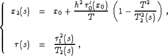 |
(42) |
where the function
 is defined by
|  |
(43) |
|  |
(44) |
and
|  |
(45) |
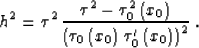
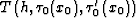
The last step of the cascade of inverse DMO, residual NMO, and DMO is
illustrated in Figure 5. The three plots in the figure show the
offset continuation to zero offset of the inverse DMO impulse response
shifted by the residual NMO operator. The middle plot corresponds to zero NMO shift, for which the DMO step collapses the wavefront back to a point.
Both positive (top plot) and negative (bottom plot) NMO shifts
result in the formation of the specific triangular impulse
response of the residual NMO+DMO operator. As noticed by Etgen
1990, the size of the ``triangle'' operators
dramatically decreases with the time increase. For large times
(pseudo-depths) of the initial impulses, the operator collapses to a
point corresponding to the pure NMO shift. This fact agrees with the
conclusions of the preceding subsection about the comparative
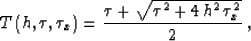
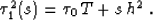
importance of the residual DMO term. It is illustrated in Figure
6 with the theoretical impulse response curves, and in
Figure 7 with the result of an actual cascade of the inverse
DMO, residual NMO, and DMO operators.
vlcvoc
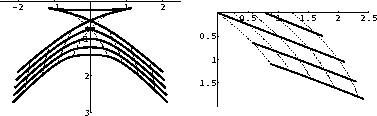
Figure 5 Kinematic residual NMO+DMO
operators constructed by the cascade of inverse DMO, residual NMO, and
DMO. The impulse response of inverse DMO is shifted by the residual
DMO procedure. Offset continuation back to zero offset forms the
impulse response of the residual NMO+DMO operator. Solid lines denote
traveltime curves; dashed lines denote the offset continuation
trajectories (time rays). Top plot: v1/v0 = 1.2. Middle plot:
v1/v0 = 1; the inverse DMO impulse response collapses back to the
initial impulse. Bottom plot: v1/v0 = 0.8. The half-offset h in
all three plots is 1 km.
|
|  |


 vlcvcp
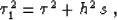
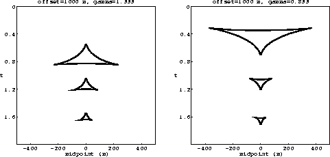
Figure 6 Theoretical
kinematics of the residual NMO+DMO impulse responses for three
impulses. Left plot: the velocity ratio v1/v0 is 1.333. Right
plot: the velocity ratio v1/v0 is 0.833. In both cases the
half-offset h is 1 km.
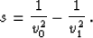
vlccps
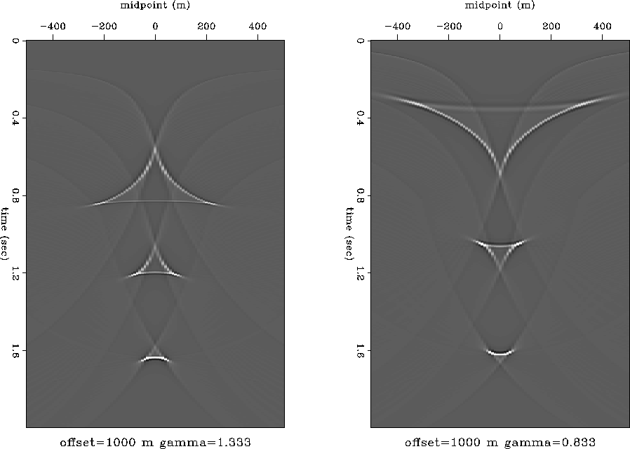
Figure 7 The result of
residual NMO+DMO (cascading inverse DMO, residual NMO, and DMO) for
three impulses. Left plot: the velocity ratio v1/v0 is
1.333. Right plot: the velocity ratio v1/v0 is 0.833. In both
cases the half-offset h is 1 km.
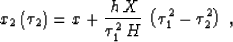
Figure 8 illustrates the residual NMO+DMO velocity
continuation for two particularly interesting cases. The left plot
shows the continuation for a point diffractor. One can see that when
the velocity error is large, focusing of the velocity rays forms a
specific loop on the zero-offset hyperbola. The right plot illustrates
the case of a plane dipping reflector. The image of the reflector
shifts both vertically and laterally with the change in NMO
velocity.
vlcvrd
Figure 8 Kinematic
velocity continuation for residual NMO+DMO. Solid lines denote
wavefronts: zero-offset traveltime curves; dashed lines denote
velocity rays. Left plot: the case of a point diffractor; the velocity
ratio v1/v0 changes from 0.9 to 1.1. Right plot:
the case of a dipping plane reflector; the velocity
ratio v1/v0 changes from 0.8 to 1.2. In both cases, the
half-offset h is 2 km.
The full residual migration operator is the result of cascading
residual zero-offset migration and residual NMO+DMO. I illustrate the
kinematics of this operator in Figures 9 and 10,
which are designed to match Etgen's Figures 2.4 and 2.5
Etgen (1990). A comparison with Figures 3 and
4 shows that including the residual DMO term affects
the images of shallow objects (with the depth smaller than the offset
h) and complicates the residual migration operator with cusps.
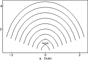
vlcve3
Figure 9 Summation paths of prestack
residual migration for a series of depth diffractors. Residual
slowness v/vd is 1.2; offset h is 1 km. This figure reproduces
Etgen's Figure 2.4.
|
|  |
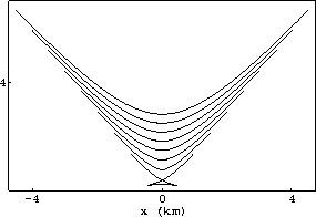
vlcve4
Figure 10 Summation paths of prestack
residual migration for a series of depth diffractors. Residual
slowness v/vd is 0.8; offset h is 1 km. This figure reproduces
Etgen's Figure 2.5.
|
|  |
Next: FROM KINEMATICS TO DYNAMICS
Up: KINEMATICS OF VELOCITY CONTINUATION
Previous: Kinematics of Residual NMO
Stanford Exploration Project
9/12/2000