|
mesh
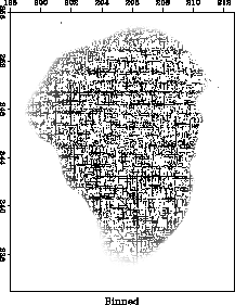
Figure 6 The Sea of Galilee dataset after a nearest-neighbor binning. The binned data is used as an input for the missing data interpolation program. |  |
I chose the familiar Galilee dataset Claerbout (1999); Fomel and Claerbout (1995) for a simple interpolation illustration. The data was collected on a bottom sounding survey of the Sea of Galilee in Israel Ben-Avraham et al. (1990). The data contain a number of noisy, erroneous and inconsistent measurements, which present a challenge for the traditional estimation methods. Addressing this challenge completely goes beyond the scope of this paper.
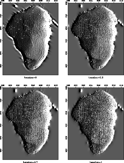
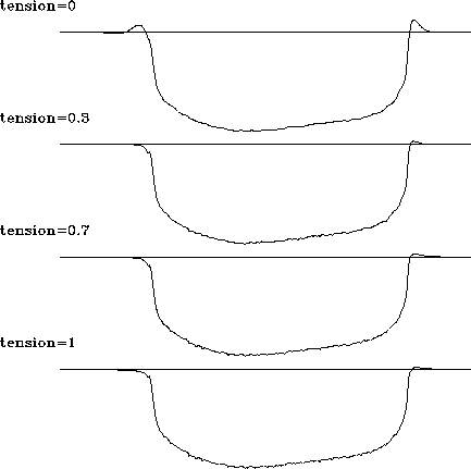
Figure 6 shows the data after a nearest-neighbor binning to a regular grid. The data was then passed to an interpolation program to fill the empty bins. The results (for different values of t) are shown in Figures 7 and 8. Interpolation with the minimum-phase Laplacian (t=0) creates a relatively smooth interpolation surface but plants artificial little mountains around the edge of the sea. This effect is caused by large gradient changes and is similar to the sidelobe effect in the one-dimensional example (Figure 2). It is clearly seen in the cross-section plots in Figure 8. Interpolation with the helix derivative (t=1) is free from the sidelobe artifacts, but it also produces an undesirable non-smooth behavior in the middle part of the image. As in the one-dimensional example, intermediate tension allows us to achieve a compromise: smooth interpolation in the middle and constrained behavior at the sides of the sea bottom.
|
mesh
Figure 6 The Sea of Galilee dataset after a nearest-neighbor binning. The binned data is used as an input for the missing data interpolation program. |  |
 |
![[*]](http://sepwww.stanford.edu/latex2html/movie.gif)
 |