

Next: Applying filter
Up: HOW TO SMOOTH RADIALLY
Previous: Constructing a filter
The number of adjustable parameters in the filter construction
is both a curse and a blessing. Whenever you add parameters to
your problem, the model space that you have to search increases
exponentially. With two adjustable parameters, taken to the extreme, at
every model point, the task can seem daunting. Generally, the
smartest course is to keep these two parameters constant throughout
the whole model space. But, this freedom also opens up interesting
possibilities. In certain regions of the data you might feel that
the radial assumption is not quite is valid, or that dips aren't changing
quite as fast. In this region you could consider making your triangle
bigger, smoothing you filter coefficients over a wider angle range, while
keeping it small in areas where dip changes quickly. The sum of the
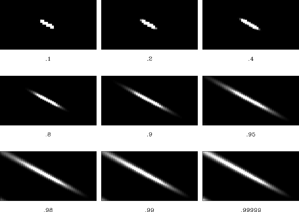
non-zero lag coefficients opens up another intriguing freedom. As
Figure 8 shows, when the sum of the non-zero lag coefficients
gets close to -1, the area over which the smoother operates increases
greatly. This is similar to increasing the  value over
only a portion of your model space. This gives you the freedom to
easily smooth regions where filter stability is questionable, while
allowing high frequency changes in areas of good data.
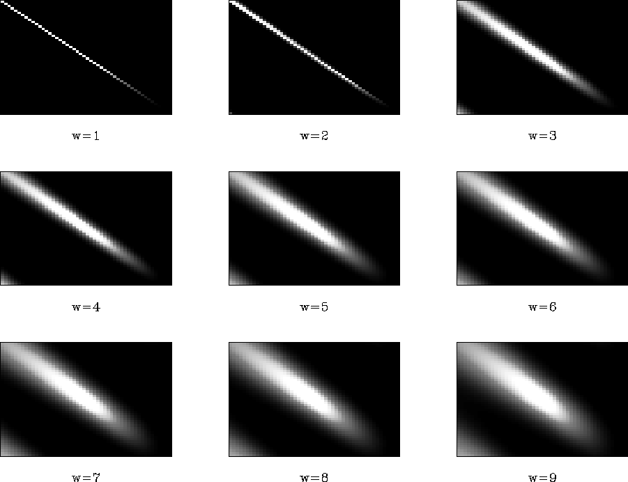
width
Figure 7 The impulse response of the smoothing filter as
function of the triangle base. Note the wider the base, the less precise
the dip smoothing.


 distance
Figure 8 The impulse response of the smoothing filter as
the sum of the non-zero lag coefficients get closer to 1.


Next: Applying filter
Up: HOW TO SMOOTH RADIALLY
Previous: Constructing a filter
Stanford Exploration Project
5/1/2000
![]() value over
only a portion of your model space. This gives you the freedom to
easily smooth regions where filter stability is questionable, while
allowing high frequency changes in areas of good data.
value over
only a portion of your model space. This gives you the freedom to
easily smooth regions where filter stability is questionable, while
allowing high frequency changes in areas of good data.

