Next: CHOOSING SMOOTHING DIRECTIONS
Up: Clapp, et al.: Radial
Previous: INTRODUCTION
Dips change quickly along every axis in seismic data. As a result a single
PEF has trouble characterizing it, even in small
patches Crawley (1999).
By estimating a space-varying PEF, we can overcome this deficiency.
Unfortunately, this changes our estimation problem from something
overdetermined to something, at times, grossly underdetermined.
To stabilize our filter estimation we must apply some type of regularization
to the standard PEF estimation optimization goals:
|  |
(1) |
| |
where  is our space-varying filter,
  is convolution with
our data, and
is convolution with
our data, and  is a roughener.
To speed up convergence, we can take advantage of helix theory Claerbout (1998c)
and reformulate our regularized problem into a preconditioned one
is a roughener.
To speed up convergence, we can take advantage of helix theory Claerbout (1998c)
and reformulate our regularized problem into a preconditioned one
|  |
(2) |
| |
where
|  |
(3) |
Our choice for can have significant influence on both
the speed and quality of our filter estimation.
The character of seismic data itself gives
us a clue on what type of regularization we should use.
A PEF filter is most successful when the statistics of the data it is
being estimated from are stationary. Logically, our rougher ,or  , should tend to smooth along a region with consistent
dips, or along Snell traces Claerbout (1978).
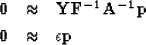
Figure 1 shows several constant velocity hyperbolas, with
the same dips highlighted. These dips all fall along a radial line through
zero time and zero offset. If we look at hyperbolas in v(z),
Figure 2, we see that there is deviation from a simple line,
but generally this trend is preserved.
, should tend to smooth along a region with consistent
dips, or along Snell traces Claerbout (1978).
Figure 1 shows several constant velocity hyperbolas, with
the same dips highlighted. These dips all fall along a radial line through
zero time and zero offset. If we look at hyperbolas in v(z),
Figure 2, we see that there is deviation from a simple line,
but generally this trend is preserved.
dips.constant
Figure 1 Constant velocity curves. The thick lines
are the same dip on all the reflectors. Note how they form a line.
|
| 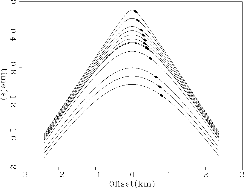 |


dips.vz
Figure 2 V(z) medium curves. The thick
lines represent the same dip. Note how they are not perfectly linear
but generally lay along a line.
|
|  |
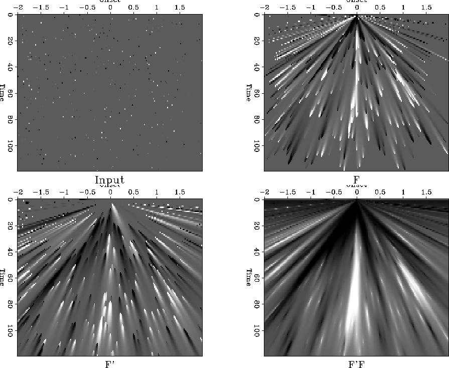
random
Figure 3 The effect of dip smoothing. The top-left panel
is the input, the top-right is the result of applying the forward operator,
bottom-left is the adjoint response; and bottom-right is the cascade of
forward and the adjoint.
Next: CHOOSING SMOOTHING DIRECTIONS
Up: Clapp, et al.: Radial
Previous: INTRODUCTION
Stanford Exploration Project
5/1/2000