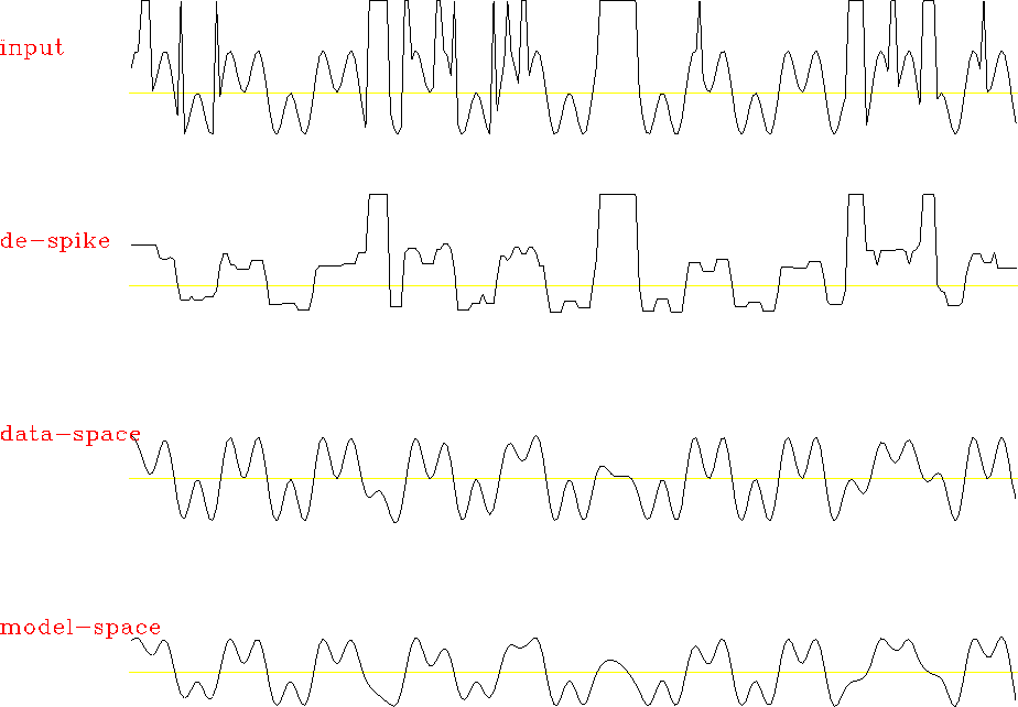
The next example of regularization is the problem of removing large spiky noise from experimental data. The input synthetic data, shown in the top plot of Figure 8, contains numerous noise spikes and bursts. Some of the noise bursts are a hundred times larger than shown. Simple median smoothing (second top plot in Figure 8) can remove some individual spikes, but fails to provide an adequate output overall. Claerbout suggests iteratively reweighted least squares as a robust efficient method of despiking. The operator L in this case is as simple as identity, but we weight equation (1) by some weighting operator W, which is chosen to suppress non-Gaussian statistical distribution of the noise. Good results in the considered example were achieved with the ``Cauchy'' weighting function
 |
(29) |
 |
Claerbout's model-space regularization used convolution with the
Laplacian filter (1,-2,1) as the roughening
operator D. For a comparison with the data-space regularization, I
applied triangle smoothing as the preconditioning operator P. The
results, shown in the two bottom plot of Figure 8, look
similar. Both methods succeeded in removing the noise bursts from the
data and producing a smooth output. The data-space regularization did
a better job of preserving the amplitudes of the original data. This
effect partially results from a low dependency on the scaling
parameter ![]() , which I reduced to 0.01 (compared
with 1 in the case of model-space regularization.) The
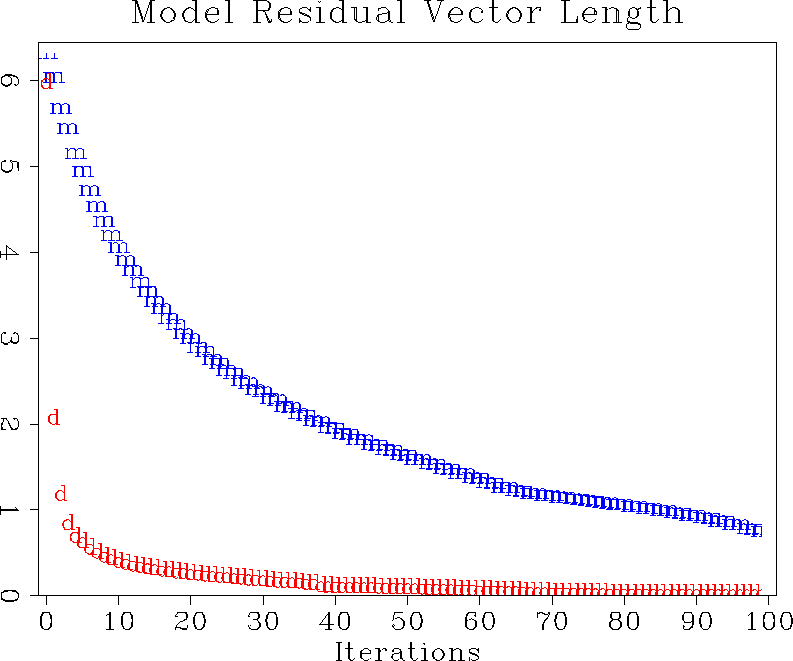
model residual plot in Figure 9 shows again a
considerably faster convergence for the data-space method, in complete
agreement with the theory.
, which I reduced to 0.01 (compared
with 1 in the case of model-space regularization.) The
model residual plot in Figure 9 shows again a
considerably faster convergence for the data-space method, in complete
agreement with the theory.
|
conv4
Figure 9 Convergence of the iterative optimization for deburst, measured in terms of the model residual. The ``d'' points stand for data-space regularization; the ``m'' points, model-space regularization. |  |