

Next: Estimating plane waves
Up: Fomel: 3-D plane waves
Previous: Introduction
Let us denote the coordinates of a three-dimensional space by t,
x, and y. A theoretical plane wave is described by the equation
|  |
(1) |
where f is an arbitrary function, and px and py are the plane
slopes in the corresponding direction. It is easy to verify that a
plane wave of the form (1) satisfies the following system
of partial differential equations:
|  |
(2) |
The first equation in (2) describes plane waves on the
 slices. In the discrete form, it can be represented as a
convolution with a two-dimensional finite-difference filter
 . Similarly, the second equation transforms into a
convolution with filter
  , which acts on the
  slices. The discrete form of equations (2) involves a
blocked convolution operator:
|  |
(3) |
In many applications, we are actually interested in the spectrum of
the prediction filter, which approximates the inverse spectrum of the
predicted data. In other words, we deal with the square operator
|  |
(4) |
If we were able to transform this operator to the form
 , where
  is a three-dimensional
minimum-phase convolution, we could use the three-dimensional filter
 in place of the inconvenient pair of
  and
and
 .
.
The problem of finding  from its spectrum is known as
spectral factorization. It is well understood for 1-D signals
Claerbout (1976), but until recently it was an open problem in
the multidimensional case. Helix transform maps multidimensional
filters to 1-D by applying special boundary conditions and allows us
to use the full arsenal of 1-D methods, including spectral
factorization, on multidimensional problems Claerbout (1998b). A problem,
analogous to (4), has already occurred in the factorization
of the discrete two-dimensional Laplacian operator:
|  |
(5) |
where  and
and  represent the partial derivative
operators along the x and y dimensions, respectively, and the
two-dimensional filter
  has been named helix
derivative Claerbout (1999); Zhao (1999).
If we represent the filter  with the help of a simple first-order
upwind finite-difference scheme
|  |
(6) |
then, after the helical mapping to 1-D, it becomes a one-dimensional
filter with the Z-transform
|  |
(7) |
where Nt is the number of samples on the t-axis. Similarly, the
filter  takes the form
|  |
(8) |
The problem is reduced to a 1-D spectrum factorization of
|  |
|
| |
| |
| (9) |
After a minimum-phase factor of (9) has been found, we can
use it for 3-D forward and inverse convolution.
All examples in this paper actually use a slightly more sophisticated
formula for 2-D plane-wave predictors:
|  |
(10) |
Formula (10) corresponds to the Lax-Wendroff finite
difference scheme Clapp et al. (1997). It provides a valid
approximation of the plane-wave differential equation for
 .
.
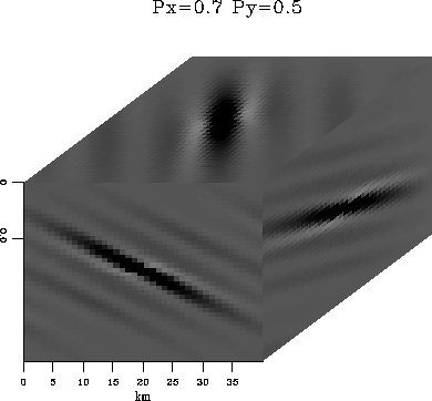
eplane
Figure 1 3-D plane wave prediction with a 402-point
filter. Left: px=0.7, py=0.5. Right: px=-0.7, py=0.5.


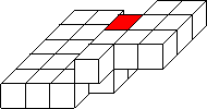
shape
Figure 2 Schematic filter shape for a 26-point 3-D
plane prediction filter. The dark block represents the leading
coefficient. There are 9 blocks in the first row and 17 blocks in
the second row.
|
|  |
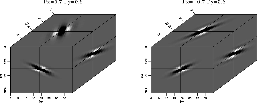
 tplane
Figure 3 3-D plane wave prediction with a 26-point
filter. Left: px=0.7, py=0.5. Right: px=-0.7, py=0.5.


Figure 1 shows examples of plane-wave construction. The
two plots in the figure are outputs of a spike, divided recursively
(on a helix) by  , where
  is a 3-D
minimum-phase filter, obtained by Wilson-Burg factorization. The
factorization was carried out in the assumption of Nt=20 and
Nx=20; therefore, the filter had Nt Nx +2 = 402 coefficients.
Using such a long filter may be too expensive for practical purposes.
Fortunately, the Wilson-Burg method allows us to specify the filter
length and shape beforehand. By experimenting with different filter
shapes, I found that a reasonable accuracy can be achieved with a
26-point filter, depicted in Figure 2. Plane-wave
construction for a shortened filter is shown in
Figure 3. The predicted plane wave is shorter and looks
more like a slanted disk. It is advantageous to deal with short plane
waves if the filter is applied for local prediction of non-stationary
signals.
In the next sections, I address the problem of estimating plane-wave
slopes and show some examples of applying local plane-wave prediction
in 3-D problems.


Next: Estimating plane waves
Up: Fomel: 3-D plane waves
Previous: Introduction
Stanford Exploration Project
5/1/2000

![]() slices. In the discrete form, it can be represented as a
convolution with a two-dimensional finite-difference filter
slices. In the discrete form, it can be represented as a
convolution with a two-dimensional finite-difference filter
![]() . Similarly, the second equation transforms into a
convolution with filter
. Similarly, the second equation transforms into a
convolution with filter ![]() , which acts on the
, which acts on the ![]() slices. The discrete form of equations (2) involves a
blocked convolution operator:
slices. The discrete form of equations (2) involves a
blocked convolution operator:
![]() from its spectrum is known as
spectral factorization. It is well understood for 1-D signals
Claerbout (1976), but until recently it was an open problem in
the multidimensional case. Helix transform maps multidimensional
filters to 1-D by applying special boundary conditions and allows us
to use the full arsenal of 1-D methods, including spectral
factorization, on multidimensional problems Claerbout (1998b). A problem,
analogous to (4), has already occurred in the factorization
of the discrete two-dimensional Laplacian operator:
from its spectrum is known as
spectral factorization. It is well understood for 1-D signals
Claerbout (1976), but until recently it was an open problem in
the multidimensional case. Helix transform maps multidimensional
filters to 1-D by applying special boundary conditions and allows us
to use the full arsenal of 1-D methods, including spectral
factorization, on multidimensional problems Claerbout (1998b). A problem,
analogous to (4), has already occurred in the factorization
of the discrete two-dimensional Laplacian operator:
![]() with the help of a simple first-order
upwind finite-difference scheme
with the help of a simple first-order
upwind finite-difference scheme


![]() , where
, where ![]() is a 3-D
minimum-phase filter, obtained by Wilson-Burg factorization. The
factorization was carried out in the assumption of Nt=20 and
Nx=20; therefore, the filter had Nt Nx +2 = 402 coefficients.
Using such a long filter may be too expensive for practical purposes.
Fortunately, the Wilson-Burg method allows us to specify the filter
length and shape beforehand. By experimenting with different filter
shapes, I found that a reasonable accuracy can be achieved with a
26-point filter, depicted in Figure 2. Plane-wave
construction for a shortened filter is shown in
Figure 3. The predicted plane wave is shorter and looks
more like a slanted disk. It is advantageous to deal with short plane
waves if the filter is applied for local prediction of non-stationary
signals.
is a 3-D
minimum-phase filter, obtained by Wilson-Burg factorization. The
factorization was carried out in the assumption of Nt=20 and
Nx=20; therefore, the filter had Nt Nx +2 = 402 coefficients.
Using such a long filter may be too expensive for practical purposes.
Fortunately, the Wilson-Burg method allows us to specify the filter
length and shape beforehand. By experimenting with different filter
shapes, I found that a reasonable accuracy can be achieved with a
26-point filter, depicted in Figure 2. Plane-wave
construction for a shortened filter is shown in
Figure 3. The predicted plane wave is shorter and looks
more like a slanted disk. It is advantageous to deal with short plane
waves if the filter is applied for local prediction of non-stationary
signals.