Continuous Fourier basis

For the continuous Fourier transform, the set of basis functions is defined by  

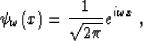$$\psi_\omega (x) = \frac{1}{\sqrt{2 \pi}} e^{i \omega x} \;,$$ (15)

where $\omega$ is the continuous frequency. For a 1-point sampling interval, the frequency is limited by the Nyquist condition: $\vert\omega\vert \leq \pi$. In this case, the interpolation function W can be computed from formula (13) to be  

$$W (x, n) = \frac{1}{2 \pi} \int_{-\pi}^{\pi} e^{i \omega (x... ...\omega = \frac{\sin \left[\pi (x - n) \right]}{\pi (x - n)} \;.$$ (16)

The interpolation function (19) is well-known as the Shannon sinc interpolator. A known problem with its practical implementation is the slow decay with (x - n). This problem is solved in practice with heuristic tapering Hale (1980), such as Harlan's triangle tapering Harlan (1982). While the function W from equation (19) automatically satisfies properties (3) and (17), where both x and n range from $-\infty$ to $\infty$, its tapered version may require additional normalization.