Accuracy

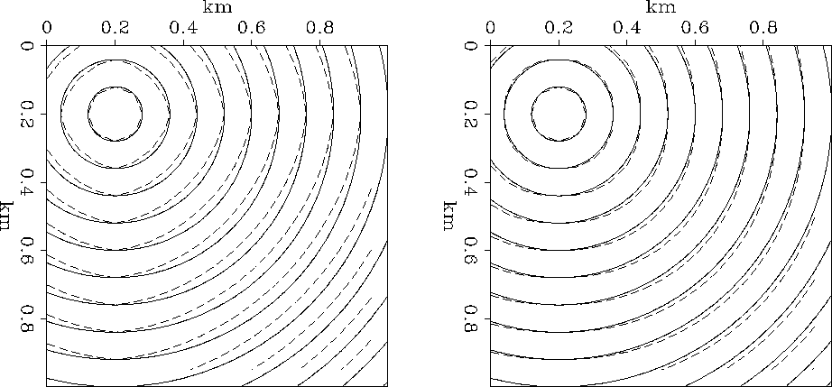
Figure 1 shows traveltime contour maps computed with the first and second-order fast marching methods on a sparse ($20 \times 20$) grid. The large errors for waves propagating at 45 to the grid are visibly reduced by the second-order formulation.

 

circles
Figure 1 Traveltime contours in a constant velocity medium. The solid line shows the exact result. The dashed line shows the first-order (left panel) and second-order (right panel) fast marching results, calculated on a $20 \times 20$ grid.

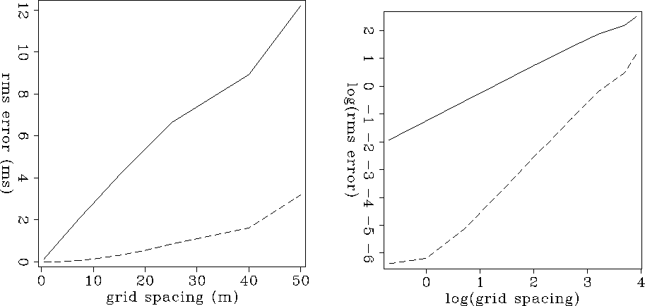
Figure 2 shows the average error as a function of grid spacing for the first and second-order solvers. Not only is the second-order formulation more accurate at large grid spacing, but its accuracy increases more rapidly as grid spacing decreases. Theory predicts the $\log-\log$ plots of average error against grid spacing to be a linear function with gradient of one for first-order methods, and two for second order methods. In practice, the fast marching results come very close to these criteria up to the limits of machine precision. Figure 2 demonstrates the superiority of the second-order fast marching formulation.

It is worth noting, at this point, that special treatment is required at the source location, since the singularity in wavefront curvature will cause numerical errors to propagate into the traveltime solution. We surround the source with a constant velocity box, within which we calculate traveltimes by ray-tracing. Errors are inversely proportional to the radius of this box. Therefore, if the radius of the box decrease with grid spacing, errors will increase linearly, reducing the accuracy of the method to first-order. For full second-order accuracy, the box size should be independent of grid spacing.

 

error
Figure 2 Average error against grid spacing for a constant velocity model. The solid line corresponds to the first-order eikonal solver, and the dashed line corresponds to the second-order solver. The left panel has linear axes, whereas the right panel is a $\log-\log$ plot.

 

marmousi
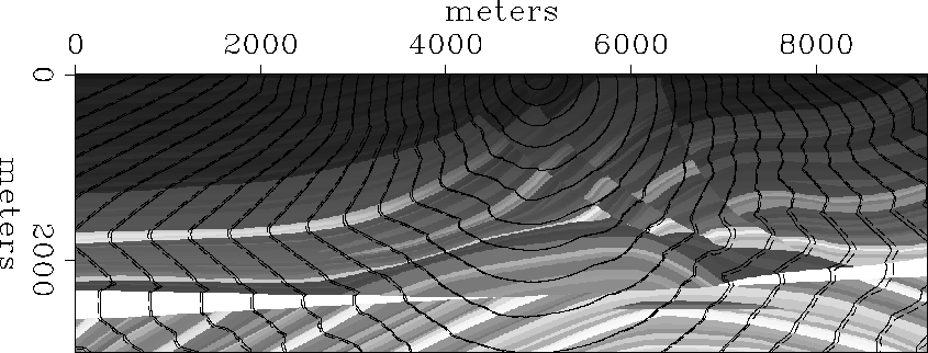
Figure 3 Traveltime contours calculated through the Marmousi velocity model sampled at 4 m. Solid line shows first-order results, and dashed line shows second-order results.