Triangulation of Height Fields

Often, a velocity field (or other object that we want to triangulate) is defined on a regular Cartesian grid. One way to perform a triangulation in this case is to select a smaller subset of the initial grid points, using them as the input to a triangulation program. We need to select the points in a way that preserves the main features of the original image, while removing some unnecessary redundancy in the regular grid description.

 

sphere
Figure 10 Illustration of Garland's algorithm for triangulation of height fields. The left plot shows the input image of a sphere, containing 100 by 100 pixels. The middle plot shows 500 pixels, selected by the algorithm and triangulated. The right plot is the result of local plane interpolation of the triangulated surface.

Garland and Heckbert 1996 surveyed different approaches to this problem and proposed a fast version of the incremental greedy insertion algorithm. Their algorithm adds points incrementally, selecting at each step the point with the maximum interpolation error with respect to the current triangulation. Though a straightforward implementation of this idea would lead to an unacceptably slow algorithm, Garland and Heckbert have discovered several sources for speeding it up. First, we can take advantage of the fact that only a small area of the current triangulation gets updated at each step. Therefore, it is sufficient to recompute the interpolation error only inside this area. Second, the maximum extraction procedure can be implemented very efficiently with a priority queue data structure.

 

opengl Figure 11 An image from the previous example, as rendered by the OpenGL library. The shades on polygonal (triangulated) sides are exaggerated by a simulation of the direct light source.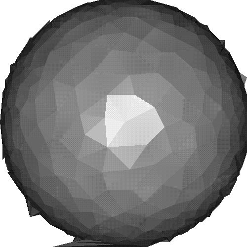

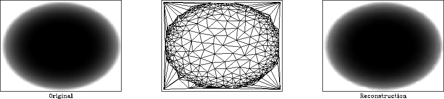
Figure 10 illustrates this algorithm with a simple example. The original image (the left plot) contained 10,000 points, laid out on a regular rectangular grid. The algorithm selects a smaller number of points and immediately triangulates them (the middle plot). The image can be reconstructed by local plane interpolation (the right plot.) The reconstruction quality can be further improved by increasing the number of triangles. Figure 11 shows the same image as rendered by the OpenGL graphics library Woo et al. (1997).

 

marmousi
Figure 12 Applying the height triangulation algorithm to the Marmousi model. The left plot shows a smoothed and windowed version of the Marmousi model. The middle plot is a result of 10,000-point triangulation, followed by linear interpolation. The right plot shows the difference between the two images.

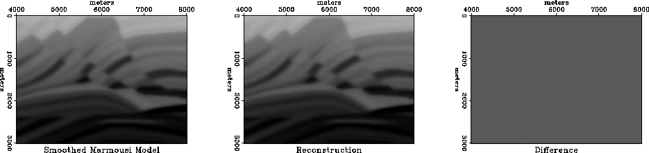Figure 12 shows an application of the height triangulation algorithm to the famous Marmousi model. The left plot shows a smoothed and windowed version of the Marmousi, plotted on a 501 by 376 computational grid. In the middle plot, 10,000 points from the original 188,376 were selected for triangulation and interpolated back to the rectangular grid. The right plot demonstates the small difference between the two images.