


Next: 2-D AMO operator
Up: Biondi, Fomel & Chemingui:
Previous: 2-D AMO operator
IN THE TIME-SPACE DOMAIN
In this appendix, we present an alternative derivation of the AMO
operator. The entire derivation is carried out in the time-space
domain. It applies the idea of cascading DMO and inverse DMO,
developed in appendix A, but uses the integral
formulation of DMO
Deregowski and Rocca (1981); Deregowski (1986); Hale (1991)
in place of the frequency-domain DMO.
Let  be the input of an AMO
operator (common-azimuth and common-offset seismic
reflection data after normal moveout correction) and
be the input of an AMO
operator (common-azimuth and common-offset seismic
reflection data after normal moveout correction) and
 be the output. Then the
three-dimensional AMO operator takes the following general form:
be the output. Then the
three-dimensional AMO operator takes the following general form:
|  |
(39) |
where  is the differentiation operator
(equivalent to multiplication by
is the differentiation operator
(equivalent to multiplication by  in the frequency domain),
 is the difference vector between the input
and the output midpoints,
is the difference vector between the input
and the output midpoints,  is the summation path,
and w12 is the weighting function.
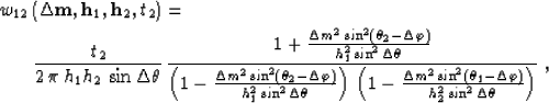
To derive (40) in the time-space domain we cascade
an integral DMO operator of the form
is the summation path,
and w12 is the weighting function.
To derive (40) in the time-space domain we cascade
an integral DMO operator of the form
|  |
(40) |
with an inverse DMO of the form
|  |
(41) |
Where  and
and  are the
summation paths of the DMO and inverse DMO operators
Deregowski and Rocca (1981):
are the
summation paths of the DMO and inverse DMO operators
Deregowski and Rocca (1981):
|  |
(42) |
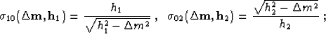
w10 and w02 are the corresponding weighting functions
(amplitudes of impulse responses);
 is the component of
 along the
  azimuth;
  is the component
of
is the component
of  along the
  azimuth;
and
azimuth;
and  ,
,  .
.  stands for the operator of half-order
differentiation (equivalent to the
stands for the operator of half-order
differentiation (equivalent to the  multiplication in
Fourier domain).
multiplication in
Fourier domain).
Both DMO and inverse DMO operate as 2-D operators on 3-D seismic data,
because their apertures are defined on a line.
This implies that for a
given input midpoint , the corresponding location of must belong to the line going through , with the azimuth
 defined by the input offset . Similarly, must be on the line going through
  with the azimuth
  of .These geometrical considerations lead us to the following
conclusion: For a given pair of input and output midpoints
and of the AMO operator, the corresponding midpoint
on the intermediate zero-offset gather is determined by the
intersection of two lines drawn through and in the
offset directions.
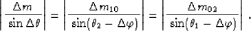
Applying the geometric connection among the three
midpoints, we can find the cascade of the DMO and inverse DMO
operators in one step. For this purpose, it is sufficient to notice
that the angles in the triangle, formed by the midpoints ,, and , satisfy the law of sines:
of .These geometrical considerations lead us to the following
conclusion: For a given pair of input and output midpoints
and of the AMO operator, the corresponding midpoint
on the intermediate zero-offset gather is determined by the
intersection of two lines drawn through and in the
offset directions.
Applying the geometric connection among the three
midpoints, we can find the cascade of the DMO and inverse DMO
operators in one step. For this purpose, it is sufficient to notice
that the angles in the triangle, formed by the midpoints ,, and , satisfy the law of sines:
|  |
(43) |
Substituting equation (41) into (42), taking
into account (44),
and neglecting the low-order asymptotic terms,
produces the 3-D integral AMO operator (40), where

| 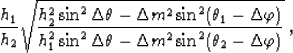 |
(44) |
|  |
(45) |
Equation (45) is the reciprocal of,
and thus equivalent to
equation (1) in the main text.
The factor
 in the denominator of the
equation (46) appears as the result
of the midpoint-coordinate transformation
in the denominator of the
equation (46) appears as the result
of the midpoint-coordinate transformation
 .
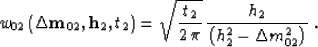
The time-and-space analogue of amplitude-preserving DMO
Black et al. (1993) has the weighting function
.
The time-and-space analogue of amplitude-preserving DMO
Black et al. (1993) has the weighting function
| 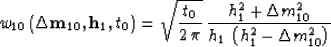 |
(46) |
while its asymptotic inverse
has the weighting function
|  |
(47) |
Inserting (47) and (48) into (46),
and using the equality 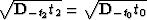 ,similarly to appendix A, yields
|  |
|
| (48) |
which is equivalent to equation (4) in the main text.
Next: 2-D AMO operator
Up: Biondi, Fomel & Chemingui:
Previous: 2-D AMO operator
Stanford Exploration Project
6/14/2000