DERIVING AMO AS A CASCADE OF DMO AND INVERSE DMO

IN THE FREQUENCY-WAVENUMBER DOMAIN

Our derivation of the AMO operator starts from the Fourier-domain formulation of DMO Hale (1984) and ``inverse'' DMO Liner (1990); Ronen (1987). However, because 3-D prestack data is often irregularly sampled, AMO is most conveniently applied as an integral operator in the time-space domain. To derive a time-space representation of the AMO impulse response from its frequency-wavenumber representation, we evaluate the stationary-phase approximation of the inverse Fourier transform along the midpoint coordinates.

The $\rm DMO$ operator and its inverse, $\rm DMO^{-1}$, can be defined in the zero-offset frequency $\omega_{0}$ and the midpoint wavenumber ${\bf k}$ as  

$$\rm DMO= \int d{t}_{1}J_1e^{-i\omega_ot_1\sqrt{1+{{\left(\frac{{{\bf k}}\cdot{{\bf h}_{1}}}{\omega_ot_1}\right)}^2}}}$$ (13)

 

$$\rm DMO^{-1}= \int d\omega_o J_2e^{+i\omega_ot_2\sqrt{1+{{\left(\frac{{{\bf k}}\cdot{{\bf h}_{2}}}{\omega_ot_2}\right)}^2}}}.$$ (14)

The $\rm AMO$ operator is given by the cascades of $\rm DMO$ and $\rm DMO^{-1}$ and its impulse response can can be written as,  

$$\rm AMO= \frac{1}{4\pi^2}\int d{{\bf k}} e^{-i{{\bf k}}\cdot... ...{\bf k}}\cdot{{\bf h}_{2}}}{\omega_ot_2}\right)}^2}}} \right)}.$$ (15)

The derivation of the stationary-phase approximation of the integral in $d{{\bf k}}$ is fairly lengthy and complex. The following outline has a similar flavor to the stationary-phase approximation of the conventional DMO impulse response presented in Black et al. (1993). We begin by changing the order of the integrals and rewriting (15) as

$$\begin{eqnarray} \rm AMO& =&\frac{1}{4\pi^2} \int dt_1 \int d\omega_o \int d{{\b... ...2 \right)-{{\bf k}}\cdot{{\bf \Delta m}} \right]}\;. \nonumber \ \end{eqnarray}$$

The phase of this integral is,  

$$\Phi\equiv \omega_o(t_1\eta_1-t_2\eta_2)-{{\bf k}}\cdot{{\bf \Delta m}},$$ (16)

where,  

$$\eta_1=\sqrt{1+{{\left(\frac{{\bf k}.{\bf h}_{1}}{\omega_ot_... ...{1+{{\left(\frac{{\bf k}.{\bf h}_{2}}{\omega_ot_2}\right)}^2}}.$$ (17)

Next we make the following change of variables and let  

$$\beta_1=\frac{{\bf h}_{1}.{\bf k}}{\omega_ot_1} \hspace{.5 i... ...pace{.5 in} \beta_2=\frac{{\bf h}_{2}.{\bf k}}{\omega_ot_2}. \ end{displaymath}$$ (18)

Therefore, $\eta_1$ and $\eta_2$ become  

$$\eta_1=\sqrt{1+\beta_1^2}\hspace{.5 in} {\rm and} \hspace{.5 in} \eta_2=\sqrt{1+\beta_2^2}.$$ (19)

The derivatives of $\eta_1$ and $\eta_2$ with respect to the in-line component of the wavenumber k_x and the cross-line component k_y can be written as

$$\begin{eqnarray} \frac{\partial{\eta_1}}{\partial{k_x}}=\frac{h_{1x}}{w_ot_1}\fr... ...ial{k_y}}=\frac{h_{2y}}{w_ot_1}\frac{\beta_2}{\sqrt{1+\beta_2^2}}.\end{eqnarray}$$ (20)

Making one more change of variables, we let  

$$\nu_1=\frac {\beta_1} {\sqrt{1+\beta_1^2}}\hspace{.5 in} {\rm and} \hspace{.5 in} \nu_2=\frac{\beta_2} {\sqrt{1+\beta_2^2}}.$$ (21)

Setting the derivative of the phase $\Phi$ to zero yields the system of equations:  

$$\left\{ \begin{array} {ll} h_{1x}\nu_1 - h_{2x}\nu_2 = \Del... ... h_{1y}\nu_1 - h_{2y}\nu_2 = \Delta m_y \end{array} \right. \ end{displaymath}$$ (22)

which we solve for $\nu_1$ and $\nu_2$ (i.e., $\eta_1$ and $\eta_2$) at the stationary path ${\bf k}_{0}$. The determinant of the system is given by  

$$\Delta=h_{2x}h_{1y}-h_{1x}h_{2y} = h_{1}h_{2}\sin \Delta \theta,$$ (23)

and the solutions for $\nu_1$ and $\nu_2$ are  

$$\nu_{01}=\frac {\Delta m\sin (\theta_{2}-\Delta \varphi)} {h_1 \sin \Delta \theta},$$ (24)

and  

$$\nu_{02}=\frac {\Delta m\sin (\theta_{1}-\Delta \varphi)} {h_2 \sin \Delta \theta}.$$ (25)

Now we need to evaluate the phase function $\Phi$ along the stationary path ${\bf k}_{0}$.By respectively multiplying the equations in (23) by k_0x and k_0y and summing them together we obtain,  

$${{\bf k}_0}\cdot{{\bf \Delta m}} = \frac{{\omega_o t_1 \beta... ...}} - \frac{{\omega_o t_2 \beta_{02}}^2}{\sqrt{1+\beta_{02}^2}}.$$ (26)

Substituting this relationship into the expression of the phase function [equation (17)] we obtain

$$\Phi_{0}= \omega_o\left(\frac{t_1}{\sqrt{1+\beta_{01}^2}}- \... ...mega_o\left(\frac{t_1}{\eta_{01}}-\frac{t_2}{\eta_{02}}\right).$$ (27)

The phase function along the stationary path is thus peaked for  

$$t_2=t_1\frac{\eta_{02}}{\eta_{01}}=t_1\frac{\sqrt{1-\nu_{01}^2}}{\sqrt{1-\nu_{02}^2}}$$ (28)

Substituting equations (25) and (26) into (29) we obtain (1) of the main text:  

$${t}_{2}= {t}_{1}\frac{h_{2}}{h_{1}}\sqrt{ \frac{h_{1}^2\sin^... ...sin^2\Delta \theta-\Delta m^2\sin^2(\theta_1-\Delta \varphi)}}.$$ (29)

Next we will derive an expression for the amplitudes of the AMO impulse response. The general expression for the stationary-phase approximation of the ${\bf k}$ integral in equation (15) is Bleistein and Handelsman (1975),  

$$A \approx \frac{2\pi J_1 J_2}{{\left\vert det\left({\bf C} \... ...f C} \!\!\!\!\! \raisebox{-.22cm}{$\sim$}\right)\frac{\pi}{4}}.$$ (30)

Therefore we need to evaluate the determinant and the signature of the curvature matrix ${\bf C} \!\!\!\!\! \raisebox{-.22cm}{$\sim$}$, which is defined as  

$${\bf C} \!\!\!\!\! \raisebox{-.22cm}{$\sim$}=\left\vert \beg... ...rac{\partial^2\Phi}{{\partial{k_y}}^2} \end{array} \right\vert.$$ (31)

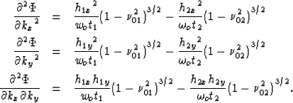
Taking the second-order partial derivatives of $\Phi$ with respect to k_x and k_y and using the definitions of $\beta_1$ and $\beta_2$ yields the following expressions for $\frac{\partial^2\Phi}{{\partial{k_x}}^2}$, $\frac{\partial^2\Phi}{{\partial{k_y}}^2}$ and $\frac{\partial^2\Phi}{\partial{k_x}\partial{k_y}}$:

$$\begin{eqnarray} \frac{\partial^2\Phi}{{\partial{k_x}}^2} & = & \frac{{h_{1x}}^2... ...^2)}^{3/2}-\frac{h_{2x}h_{2y}}{\omega_ot_2}{(1-\nu_{02}^2)}^{3/2}.\end{eqnarray}$$ (32) (33) (34)

With a little algebra, one may verify that the determinant of the curvature matrix is

$$\begin{eqnarray} det(C) & = & -\frac{\Delta^2}{\left\vert\omega_o\right\vert^2t... ...mega_o\right\vert^2t_0^2}{(1-\nu_{01}^2)}^{2}{(1-\nu_{02}^2)}^{2}.\end{eqnarray}$$ (35)

We notice that the determinant of ${\bf C} \!\!\!\!\! \raisebox{-.22cm}{$\sim$}$,which is the product of the two eigenvalues of ${\bf C} \!\!\!\!\! \raisebox{-.22cm}{$\sim$}$,is always negative, that is; that the two eigenvalues have opposite signs and thus the signature of ${\bf C} \!\!\!\!\! \raisebox{-.22cm}{$\sim$}$,which is defined as the number of positive eigenvalues minus the number of negative eigenvalues, is always null. Therefore, the second term of the phase shift in equation (31) vanishes.

To obtain expressions for the AMO amplitude, we need to substitute equation (36) in equation (31), together with the corresponding expressions for J₁ and J₂. For the Jacobian J₁ of the forward DMO we can use any of the Jacobians proposed in the literature by Hale 1984, Zhang and Black 1988, and Bleistein 1990. The Jacobian J₂ of inverse DMO can be derived with Beylkin's theory for the asymptotic inverse of stacking operators Beylkin (1985); Cohen and Hagin (1985). The expression for the Jacobian of the asymptotic inverse for Hale's DMO were derived by Liner and Cohen 1988. Chemingui and Biondi 1995 and Fowler (personal communication) independently derived the inverse for Zhang-Black's DMO. As mentioned in the main text, we used Zhang-Black's Jacobians for the actual application of AMO; that is,  

$$J_1= \frac{(1+\nu_{01}^2)}{\sqrt{1-\nu_{01}^2}}, \;\;\;\;\;\;\; J_2=1.$$ (36)

Finally, after taking into account he Jacobian of the transformation from t₁ to t₀ ($dt_1 =dt_0 {\sqrt{1-\nu_{01}^2}}$)in the first integral of equation (16), we can write the amplitude term for the AMO integral:

$$\begin{eqnarray} A & \approx & \frac{\left\vert\omega_o\right\vert t_0}{2\pi\De... ...\pi\Delta}\frac{(1+\nu_{01}^2)}{{(1-\nu_{01}^2)}{(1-\nu_{02}^2)}}.\end{eqnarray}$$ (37) (38)

The last substitution, $\left\vert\omega_o\right\vert t_0=\left\vert\omega_2\right\vert t_2$,enables us to apply the differentiation operator $\left\vert\omega_2\right\vert$ to the output data; it is correct because t₀ and t₂ are linked by the linear relationship $t_0 =t_2 {\sqrt{1-\nu_{02}^2}}$.The expression for the amplitudes presented in equation (4) of the main text follows by simple substitution of the expressions for $\Delta$, $\nu_{01}$,and $\nu_{02}$, from equations (24), (25) and  (26) into equation (39).