|
uncertain
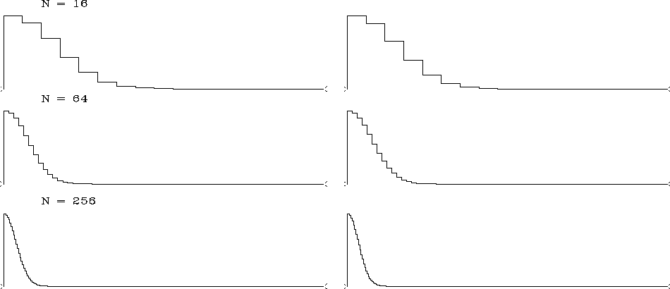
Figure 2 Sampled Gaussian functions and their Fourier transforms for vectors of length n = 16, 64, and 256. |  |
Now examine Figure 2, which contains sampled Gaussian functions and their Fourier transforms. The Fourier transform of a Gaussian is well known to be another Gaussian function, as the plot confirms. I adjusted the width of each Gaussian so that the widths would be about equal in both domains. The Gaussians were sampled at various values of n, increasing in steps by a factor of 4. You can measure the width dropping by a factor of 2 at each step. For those of you who have already learned about the uncertainty principle, it may seem paradoxical that the function's width is dropping in both time and frequency domains.
|
uncertain
Figure 2 Sampled Gaussian functions and their Fourier transforms for vectors of length n = 16, 64, and 256. |  |
The resolution of the paradox is that the
physical length of the time axis or the frequency axis
is varying as we change n
(even though the plot length is scaled to a constant on the page).
We need to associate a physical mesh with the computational mesh.
A method of associating physical and computational meshes
was described in chapter ![[*]](http://sepwww.stanford.edu/latex2html/cross_ref_motif.gif) on page
on page ![[*]](http://sepwww.stanford.edu/latex2html/cross_ref_motif.gif) .
In real physical space as well as in Fourier transform space,
the object remains a constant size as the mesh is refined.
.
In real physical space as well as in Fourier transform space,
the object remains a constant size as the mesh is refined.
Let us read from Figure 2 values for
the widths ![]() and
and ![]() .On the top row, where N=16, I pick a width of about 4 points,
and this seems to include about 90%
of the area under the function.
For this signal (with the widths roughly equal in both domains)
it seems that
.On the top row, where N=16, I pick a width of about 4 points,
and this seems to include about 90%
of the area under the function.
For this signal (with the widths roughly equal in both domains)
it seems that
![]() and
and ![]() .Using the relation between dt and df found
in equation (
.Using the relation between dt and df found
in equation (![[*]](http://sepwww.stanford.edu/latex2html/cross_ref_motif.gif) ),
which says that
),
which says that ![]() ,the product becomes
,the product becomes
![]() = 1.
= 1.
We could also confirm the inequality (1) by
considering simple functions
for which we know the analytic transforms--for example,
an impulse function in time.
Then ![]() , and the Fourier transform occupies
the entire frequency band
from minus to plus the Nyquist frequency
, and the Fourier transform occupies
the entire frequency band
from minus to plus the Nyquist frequency ![]() Hz,
i.e.,
Hz,
i.e., ![]() .Thus again, the product is
.Thus again, the product is ![]() = 1.
= 1.