


Next: THE MEANING OF THE
Up: SURVEY SINKING WITH THE
Previous: The DSR equation in
By converting the DSR equation to midpoint-offset space
we will be able to identify the familiar zero-offset migration part
along with corrections for offset.
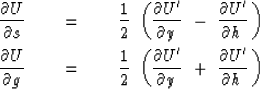
The transformation between (g,s) recording parameters
and (y,h) interpretation parameters is
| 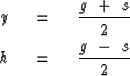 |
(37) |
| (38) |
Travel time t may be parameterized in (g,s)-space or (y,h)-space.
Differential relations for this
conversion are given by the chain rule for derivatives:
| 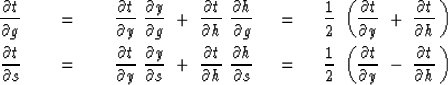 |
(39) |
| (40) |
Having seen how stepouts transform from shot-geophone space
to midpoint-offset space,
let us next see that spatial frequencies transform in much the same way.
Clearly, data could be transformed from (s,g)-space
to (y,h)-space with (37) and (38)
and then Fourier transformed to ( ky , kh )-space.
The question is then,
what form would the double-square-root equation (35)
take in terms of the spatial frequencies ( ky , kh )?
Define the seismic data field in either coordinate system as
| 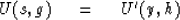 |
(41) |
This introduces a new mathematical function U' with the same
physical meaning as U but,
like a computer subroutine or function call,
with a different subscript look-up procedure
for (y,h) than for (s,g).
Applying the chain rule for partial differentiation to (41) gives
| 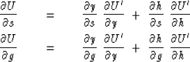 |
(42) |
| (43) |
and utilizing (37) and (38) gives
|  |
(44) |
| (45) |
In Fourier transform space
where  transforms to i kx,
equations (44) and (45),
when i and U = U' are cancelled, become
transforms to i kx,
equations (44) and (45),
when i and U = U' are cancelled, become
|  |
(46) |
| (47) |
Equations (46)
and (47)
are Fourier representations of (44) and (45).
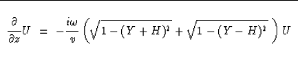
Substituting (46) and (47)
into (35) achieves the main purpose of this section,
which is to get the double-square-root migration equation
into midpoint-offset coordinates:
| ![\begin{displaymath}
{\partial\ \over \partial z} \ U\ \ =\ \ -\,i \,
{\omega \o...
..._y \,-\, v k_h \over 2\,\omega } \, \right)^2
\ } \ \right] \ U\end{displaymath}](img70.gif) |
(48) |
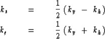
Equation (48) is the takeoff point
for many kinds of common-midpoint seismogram analyses.
Some convenient definitions that simplify its appearance are
| 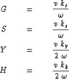 |
(49) |
| (50) |
| (51) |
| (52) |
Chapter ![[*]](http://sepwww.stanford.edu/latex2html/cross_ref_motif.gif) showed that the quantity
showed that the quantity  can
be interpreted as the angle of a wave.
Thus the new definitions S and G are the sines
of the takeoff angle and of the arrival angle of a ray.
When these sines are at their limits of
can
be interpreted as the angle of a wave.
Thus the new definitions S and G are the sines
of the takeoff angle and of the arrival angle of a ray.
When these sines are at their limits of  they refer
to the steepest possible slopes in (s,t)- or (g,t)-space.
Likewise, Y may be interpreted as the dip of the data as seen
on a seismic section.
The quantity H refers to stepout observed on a common-midpoint gather.
With these definitions (48) becomes slightly less cluttered:
they refer
to the steepest possible slopes in (s,t)- or (g,t)-space.
Likewise, Y may be interpreted as the dip of the data as seen
on a seismic section.
The quantity H refers to stepout observed on a common-midpoint gather.
With these definitions (48) becomes slightly less cluttered:
|  |
(53) |
Most present-day before-stack migration procedures
can be interpreted through
equation (53).
Further analysis of it will explain
the limitations of conventional processing procedures
as well as suggest improvements in the procedures.
EXERCISES:
-
Adapt equation (48) to allow for a difference in velocity
between the shot and the geophone.
-
Adapt equation (48) to allow for downgoing pressure waves
and upcoming shear waves.
Next: THE MEANING OF THE
Up: SURVEY SINKING WITH THE
Previous: The DSR equation in
Stanford Exploration Project
10/31/1997