Linear interpolation

The linear interpolation operator is much like the binning operator but a little fancier. When we perform the forward operation, we take each data coordinate and see which two model bin centers bracket it. Then we pick up the two bracketing model values and weight each of them in proportion to their nearness to the data coordinate, and add them to get the data value (ordinate). The adjoint operation is adding a data value back into the model vector; using the same two weights, the adjoint distributes the data ordinate value between the two nearest bins in the model vector. 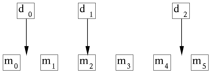For example, suppose we have a data point near each end of the model and a third data point exactly in the middle. Then for a model space 6 points long, as shown in Figure , we have the operator in (16).

 

helgerud Figure 4 Uniformly sampled model space and irregularly sampled data space corresponding to (16).

 

$$\left[ \begin{array} {c} d_0 \\ d_1 \\ d_2 \end{ar... ...m_1 \\ m_2 \\ m_3 \\ m_4 \\ m_5 \end{array}\right]$$ (16)

The two weights in each row sum to unity. If a binning operator were used for the same data and model, the binning operator would contain a ``1.'' in each row. In one dimension (as here), data coordinates are often sorted into sequence, so that the matrix is crudely a diagonal matrix like equation (16). If the data coordinates covered the model space uniformly, the adjoint would roughly be the inverse. Otherwise, when data values pile up in some places and gaps remain elsewhere, the adjoint would be far from the inverse.

Module lint1 does linear interpolation and its adjoint. In chapters and we build inverse operators. lint1linear interp