MIGRATION WITH ANTIALIASING

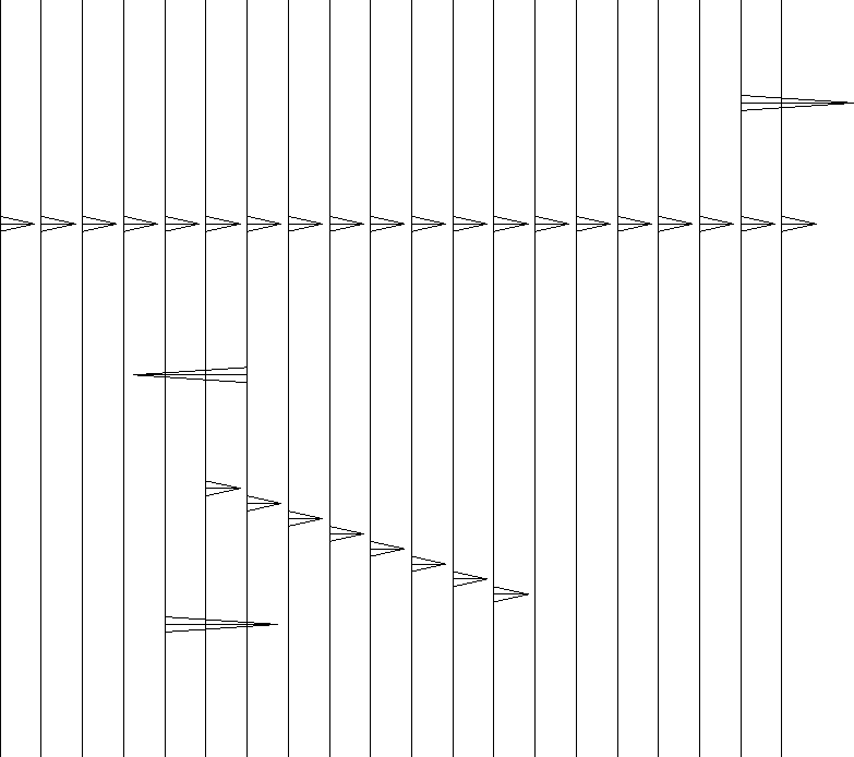Subroutine aamig() below does migration and diffraction modeling using subroutine trimo() as the workhorse.  

# anti-aliased kirchhoff migration (adj=1) and modeling (adj=0)
#
subroutine aamig( adj,add, slow,antialias,t0,dt, dx, nt,nx, image, data  )
integer adj, add, ix, nx, nt, iy
real    h,            slow(nt),antialias,t0,dt, dx, image(nt,nx), data(nt,nx)
call adjnull(    adj, add,                          image,nt*nx,  data,nt*nx)
do ix= 1, nx {
do iy= 1, nx {
        h  = dx * (iy - ix)
        call trimo( adj, 1, t0,dt,dx, h, nt,slow, 0., 1., antialias, _
                                                        image(1,iy), data(1,ix))
        }}
return; end

Figure 9 shows the synthetic image that is used for testing. There is a horizontal layer, a dipping layer, and a few impulses. The impulses are chosen stronger than the layers because they will spread out in the synthetic data.

 

aamod Figure 9 Model image for migration study.

The velocity is taken constant. Figure 10 shows synthetic data made without regard for aliasing. The hyperbolas look fine--the way we expect. The horizontal layer, however, is followed by many pseudo layers. These pseudo layers are the result of modeling with an operator that is spatially aliased.

 

aad0 Figure 10 Synthetic data without regard for aliasing. Made from model image with aamig() taking antialias=0.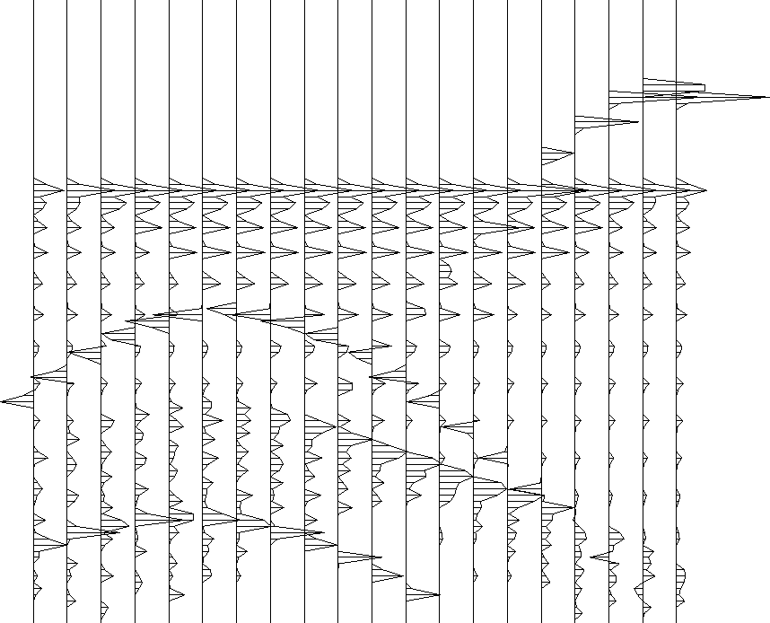

Figure 11 shows how the synthetic data improves dramatically when aliasing is taken into account. The layers look fine now. The hyperbolas, however, have a waveform that is rapidly changing with offset from the apex. This changing waveform is an inevitable consequence of the anti-aliasing. The apex has a huge amplitude because the temporal bandwidth is widest at the apex (because the dip is zero there, there is no filtering away of high spatial frequencies). Simple low-pass temporal filtering (not shown) will cause the wavelet to be largely independent of offset.

 

aad1 Figure 11 Synthetic data accounting for aliasing. Made from model image with aamig() taking antialias=1.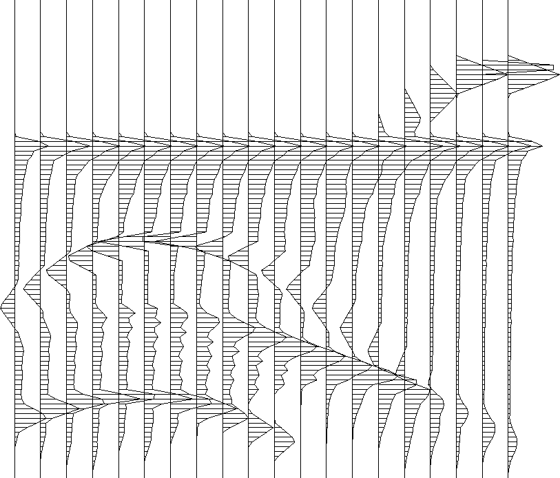

Do not confuse aliased data with synthetic data made by an aliased operator. To make aliased data, you would start from good data, such as Figure 11, and throw out alternate traces. More typically, the earth makes good data and we fail to record all the needed traces for the quality of our field arrays.

The horizontal layer in Figure 11 has a waveform that resembles a damped step function which is related to the Hankel tail we studied in chapter  where subroutine halfdifa() was introduced to provide the filter required to convert the waveform on the horizontal layer in Figure 11 back to an impulse. This was done in Figure 12. You can see the final flat-layer waveform is roughly the zero-phase shape we started with.

 

aad1h Figure 12 Best synthetic data. Made from model image using aamig() with antialias=1 followed by a causal half-order time derivative. Lowpass temporal filtering would make wavelets more independent of location on a hyperbola.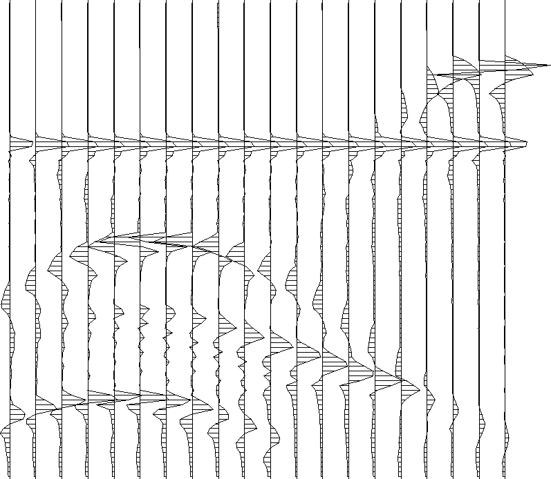

Figure 13 shows my best migration of my best synthetic data. All the features of the original model are apparent. Naturally, high frequencies are lost, more on the dipping bed than the level one. Likewise the broadening of the deeper point scatterer compared to the shallow one is a well known aperture effect.

 

aamig2 Figure 13 Best migration of best synthetic data. Uses aamig() with antialias=2 followed by an anticausal half-order time derivative.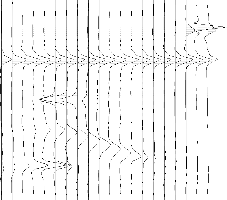

Figure 14 shows what happens when antialiasing is ignored in migration. Notice many false layers above the given horizontal layer. Notice semicircles above the impulses. Notice apparent noise everywhere. But notice also that the dipping bed is sharper than the antialiased result in Figure 13.

 

aamig0 Figure 14 Migration of best synthetic data without regard for aliasing. Uses aamig() with antialias=0. (and an anticausal half-order time derivative)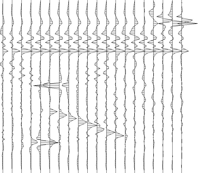