Next: Space variable filters
Up: THEORY/MOTIVATION
Previous: Helix transform
At this point a discussion of steering filters is appropriate.
Plane waves with a given slope on a discrete grid can be predicted
(destroyed) with compact filters Schwab (1997). Inverting
such a filter by the helix method, we can create a signal with a given
arbitrary slope extremely quickly. If this slope is expected in the
model, the described procedure gives us a very efficient method of
preconditioning the model estimation problem, fitting goal (2).
How can a plane prediction (steering) filter be created? On the helix surface,
the plane wave P(t,x) = f (t - p x) translates naturally into a
periodic signal with the period of  , where Nt is
the number of points on the t trace, and
, where Nt is
the number of points on the t trace, and  , where
  is the plane slope,
![[*]](http://sepwww.stanford.edu/latex2html/foot_motif.gif) and
and  and
and  correspond to the mesh size.
If we design a filter that is two columns long
(assuming the columns go in the t direction), then the plane
prediction problem is simply connected with the
interpolation problem: to destroy a plane wave, shift the
signal by T, interpolate it, and subtract the result from the
original signal. Therefore, we can formally write
correspond to the mesh size.
If we design a filter that is two columns long
(assuming the columns go in the t direction), then the plane
prediction problem is simply connected with the
interpolation problem: to destroy a plane wave, shift the
signal by T, interpolate it, and subtract the result from the
original signal. Therefore, we can formally write
|  |
(6) |
where  denotes the steering filter,
  is
the shift-and-interpolation operator, and
is
the shift-and-interpolation operator, and  is the identity
operator.
is the identity
operator.
Different choices for the operator in (6)
produce filters with different length and prediction power.
A shifting operation corresponds to the filter with the Z-transform
 , while the operator corresponds to an
approximation of
, while the operator corresponds to an
approximation of  with integer powers of Z. One possible
approach is to expand
with integer powers of Z. One possible
approach is to expand  using the Taylor series around
the zero frequency (Z=1). For example, the first-order approximation
is
using the Taylor series around
the zero frequency (Z=1). For example, the first-order approximation
is
|  |
(7) |
which corresponds to linear interpolation and leads in the
two-dimensional space to the steering filter of the
form
|  |
(8) |
Filter (8) is equivalent to the explicit first-order upwind
finite-difference scheme on the plane wave equation
| 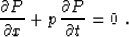 |
(9) |
An important property of filter (8) is that it produces an
exact answer for  and
and  . The values of
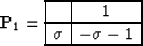
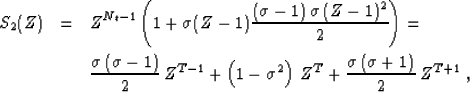
  lead to unstable inversion. For negative , the filter is
reflected:
lead to unstable inversion. For negative , the filter is
reflected:
|  |
(10) |
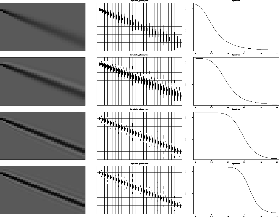
The top panel in Figure 2 shows a plane wave, created
by applying the helix inverse of filter (8) on a single
spike (unit impulse) for the value of  . We see a
noticeable frequency dispersion, caused by the low order of the
approximation.
steer-lagrange
. We see a
noticeable frequency dispersion, caused by the low order of the
approximation.
steer-lagrange
Figure 2 Steering filters with
Lagrange interpolation. The left and middle plots show the impulse
responses of steering filters: the top panel corresponds to
linear interpolation (two-point Lagrange, upwind finite-difference);
the second top plot, the three-point Lagrange filter (Lax-Wendroff
scheme); the two bottom plots, the 8-point and 13-point Lagrange
filters. The right plots in each panel show the corresponding
average spectrum. The spectrum flattens and the prediction get more
accurate with an increase of the filter size.


The second-order Taylor approximation yields
|  |
|
| (11) |
which corresponds to the 2-D filter
|  |
(12) |
and is equivalent to the Lax-Wendroff finite-difference scheme
of equation (9). The interpolation, implied by filter
(10) is a local three-point polynomial (Lagrange)
interpolation. The correspondence of the Taylor series method,
described above, and the Lagrange interpolation can be proved by
induction. In general, the filter coefficients for the second row of
the N-th order Lagrangian filter are given by the explicit formula
| ![\begin{displaymath}
a_{k} = \prod_{i \neq k} \frac{(\sigma-\left[\frac{N}{2}\right]-i)}{(k-i)}\;,\end{displaymath}](img35.gif) |
(13) |
where the k and i range from to N. Such a filter has a
stable inverse for 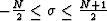 and
additionally produces an exact answer for all integer 's in
that range. We would have arrived at the same conclusion if instead of
expanding the Z-transform of the filter around Z=1,
expanded its Fourier transform around the zero frequency. The latter
case corresponds to the ``self-similar'' construction of
Karrenbach (1995). The impulse responses for the helix
inverses of different-order Lagrangian filters are shown in Figure
2.
and
additionally produces an exact answer for all integer 's in
that range. We would have arrived at the same conclusion if instead of
expanding the Z-transform of the filter around Z=1,
expanded its Fourier transform around the zero frequency. The latter
case corresponds to the ``self-similar'' construction of
Karrenbach (1995). The impulse responses for the helix
inverses of different-order Lagrangian filters are shown in Figure
2.
If instead of Taylor series in Z, we use a rational (Padè)
approximation, the filter will get more than one coefficient in the
first row, which corresponds to an implicit finite-difference scheme.
For example, the [1/1] Padè approximation is
| 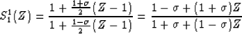 |
(14) |
which leads to the filter
| 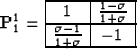 |
(15) |
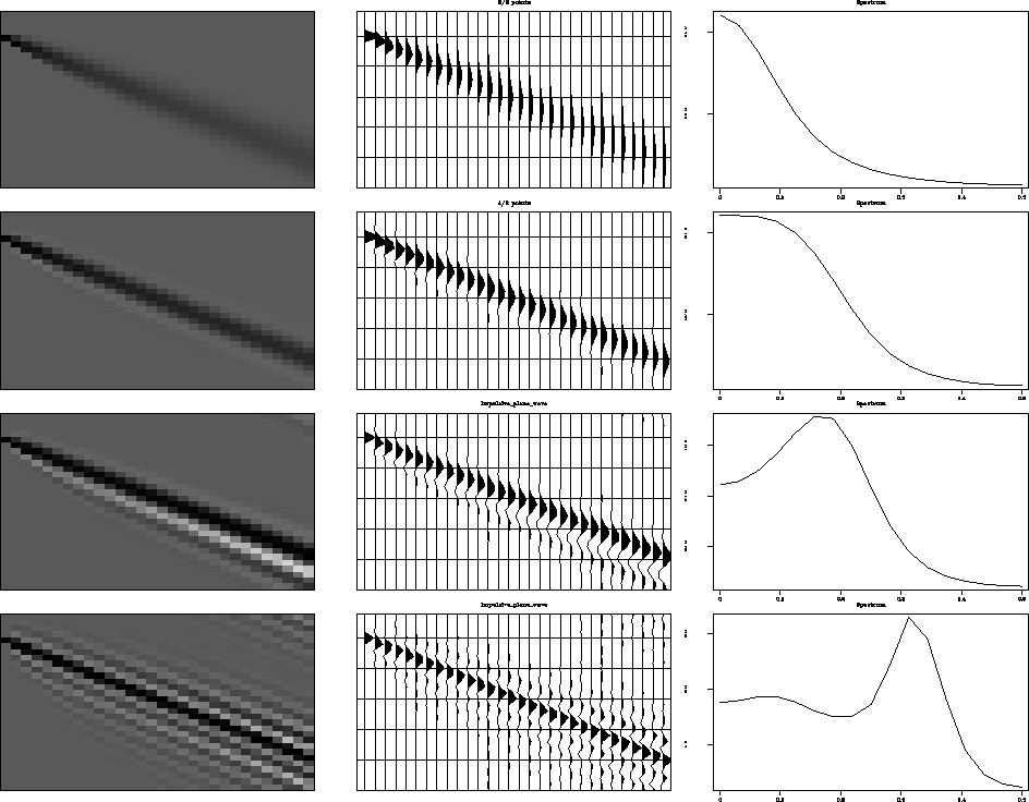
and corresponds to the Crank-Nicolson implicit scheme. The
impulse response for the inverse of filter (15) is shown in
the top plot of Figure 3. It shows some mild
improvements in comparison with the explicit Lagrangian filter of the
same order. In our experience, filters with more than one additional
coefficient in the first column behave unstably when inverted.
steer-other
Figure 3 Steering filters with
different types of interpolation. The left and middle plots show the
impulse responses of the steering filters: the top panel
corresponds to first-order Padè interpolation (Crank-Nicolson
scheme); the second top plot, the (8/2) Padè approximation; the two
bottom plots, the 8-point and 12-point Lagrange filters. The right
plots in each panel show the corresponding average spectrum.
Other types of interpolations could be used for the steering
filters Fomel (1997b) The two bottom panels of Figure
3 show the impulse responses for the filters, based on
the tapered sinc interpolation. The filters suffer from high-frequency
oscillations, but otherwise also perform well.
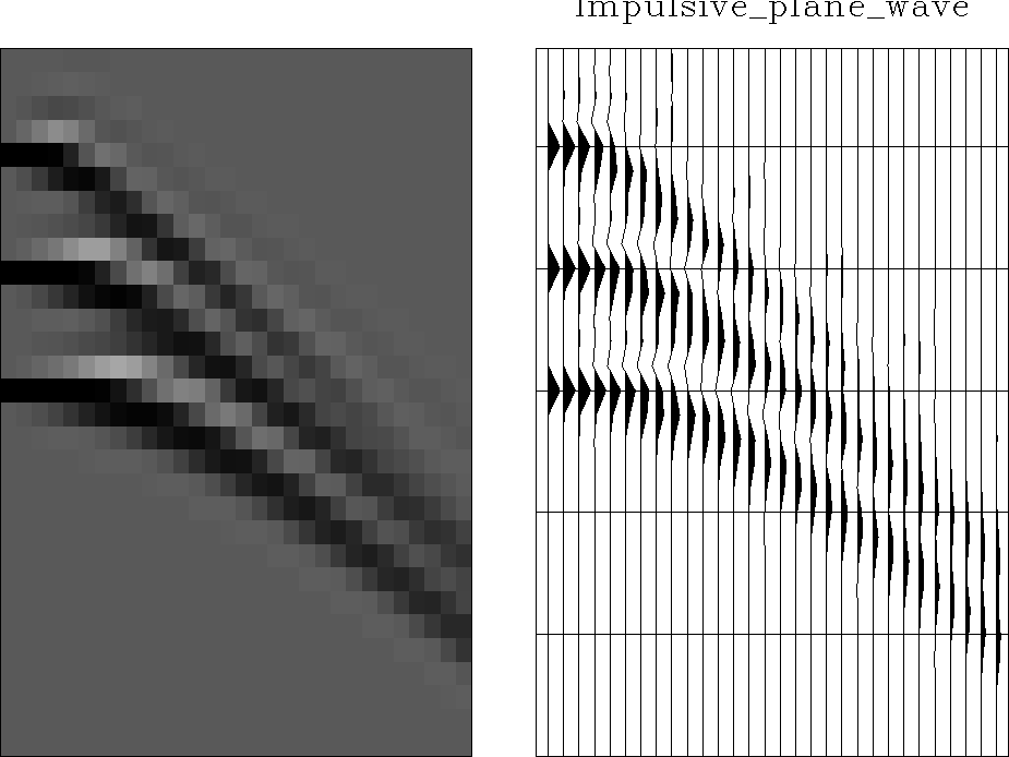
It is interesting to note that a space-variant convolution with
inverse plane filters can create signals with different shape, which
remains planar only locally. This situation corresponds to a variable
slowness p in the one-way wave equation (9). Figure
4 shows an example: predicting hyperbolas with a 7-point
Lagrangian filter.
steer-hyp7
Figure 4 Creating hyperbolas with a variant
plane-wave prediction: the impulse response of the inverse 7-point
time-and-space-variant Lagrangian filter.
Next: Space variable filters
Up: THEORY/MOTIVATION
Previous: Helix transform
Stanford Exploration Project
9/12/2000