Next: THE IMPULSE RESPONSE OF
Up: Fomel: Offset continuation
Previous: SOLVING THE CAUCHY PROBLEM
In this Appendix, I apply an alternative method to derive formula
(10), which describes the summation path of the integral OC
operator. The method is based on the following considerations.
The summation path of an integral (stacking) operator coincides with
the phase function of the impulse response of the inverse
operator. Impulse response is by definition the operator reaction to
an impulse in the input data. For the case of offset continuation, the
input is a reflection common-offset gather. From the physical point of
view, an impulse in this type of data corresponds to the special
focusing reflector (elliptical isochrone) at the depth. Therefore,
reflection from this reflector at a different constant-offset
corresponds to the impulse response of the OC operator. In other
words, we can view offset continuation as the result of cascading
prestack common-offset migration, which produces the elliptic surface,
and common-offset modeling (inverse migration) for different offsets.
This approach resemble that of Deregowski and Rocca
1981. It was applied recently to a more
general case of azimuth moveout (AMO) by Fomel and Biondi
1995. The geometric approach implies that in order to
find the summation pass of the OC operator, one should solve the
kinematic problem of reflection from an elliptic reflector, whose
focuses are in the shot and receiver locations of the output seismic
gather.
In order to solve this problem , let us consider an elliptic surface of
the general form
|  |
(66) |
where  is less than 1. In a constant velocity
medium, the reflection ray path for a given source-receiver pair on
the surface is controlled by the position of the reflection point x.
Fermat's principle provides a required constraint for finding this
position. According to Fermat's principle, the reflection ray path
corresponds to an extremum value of the travel-time. Therefore, in the
neighborhood of this path,
is less than 1. In a constant velocity
medium, the reflection ray path for a given source-receiver pair on
the surface is controlled by the position of the reflection point x.
Fermat's principle provides a required constraint for finding this
position. According to Fermat's principle, the reflection ray path
corresponds to an extremum value of the travel-time. Therefore, in the
neighborhood of this path,
|  |
(67) |
where s and r stand for the source and receiver locations on the
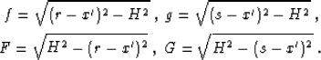
surface, and  is the reflection traveltime
|  |
(68) |
Substituting (71) and (69) into (70) leads to a
quadratic algebraic equation on the reflection point parameter x.
This equation has the explicit solution
|  |
(69) |
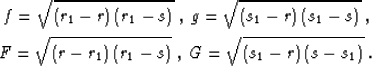
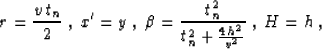
where h=(r-s)/2,  , y=(s+r)/2, and
  . Replacing x in formula (71) with its
expression (72) solves the kinematic part of the problem,
producing the explicit traveltime expression
. Replacing x in formula (71) with its
expression (72) solves the kinematic part of the problem,
producing the explicit traveltime expression
|  |
(70) |
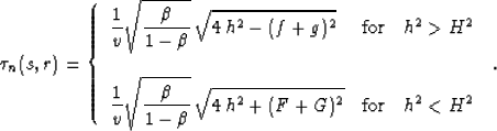
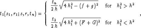
where
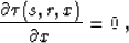
Two branches of formula (73) correspond to the difference in the
geometry of the reflected rays in two different situations. When a
source-and-receiver pair is inside the focuses of the elliptic
reflector, the midpoint y and the reflection point x are on the
same side of the ellipse with respect to its small semi-axis. They are
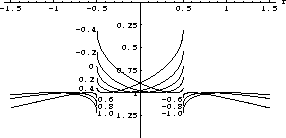
on different sides in the opposite case (Figure 5).
offell
Figure 5
Reflections from an ellipse. The three pairs of reflected rays
correspond to a common midpoint (at 0.1) and different offsets. The
focuses of the ellipse are at 1 and -1.
|
|  |


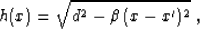
If we apply the NMO correction, formula (73) is transformed to
|  |
(71) |
Then, recalling the relationships between the parameters of the
focusing ellipse r, x' and and the parameters of the
output seismic gather Deregowski and Rocca (1981)
|  |
(72) |
and substituting expressions (75) into formula (74) yields the
expression
|  |
(73) |
where
It is easy to verify algebraically the mathematical equivalence of
equation (76) and equation (10) in the main
text. The kinematic approach described in this appendix applies
equally well to different acquisition configurations of the input and
output data. The source-receiver parameterization used in
(76) is the actual definition for the summation path of the
integral shot continuation operator Bagaini and Spagnolini (1993); Schwab (1993). A
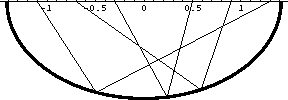
family of these summation curves is shown in Figure 6.
offshc
Figure 6
Summation paths of the integral shot continuation. The output source
is at -0.5 km. The output receiver is at 0.5 km. The indexes of the
curves correspond to the input source location.
C
Next: THE IMPULSE RESPONSE OF
Up: Fomel: Offset continuation
Previous: SOLVING THE CAUCHY PROBLEM
Stanford Exploration Project
4/19/2000