The 45 wave equation

The diffraction term of the in the 45 equation Claerbout (1985) can be rewritten as the following matrix equation, by inserting the rational part of the implicit extrapolator (3) into equation (1):

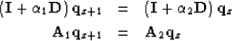$$\begin{eqnarray} \left({\bf I} + \alpha_1 {\bf D} \right) {\bf q}_{z+1} & = & \l... ... {\bf q}_{z} \\ {\bf A}_1{\bf q}_{z+1} & = & {\bf A}_2{\bf q}_{z}\end{eqnarray}$$ (5) (6)

where the complex coefficients $\alpha_1$ and $\alpha_2$ can be calculated, and ${\bf D}$ is a finite-difference representation of the Laplacian, $\nabla^2$.

The right-hand-side of equation (6) is known. The challenge is to find the vector ${\bf q}_{z+1}$ by inverting the matrix, ${\bf A}_1$.Given the wavefield on the surface, this equation provides a way to downward-continue in depth.

The matrices in equation (6) represent convolution with a scaled finite-difference Laplacian, with its main diagonal stabilized. Scaling coefficients, $\alpha_1$ and $\alpha_2$, are complex and depend on the ratio, $\omega/v$.

In the two-dimensional problem, the $\nabla^2$ operator acts only in the x-direction, and can be represented by the three-point convolutional filter, d=(1,-2,1). The matrix, ${\bf A}_1$,therefore, has a tridiagonal structure, which can be inverted efficiently with a recursive solver.

In three-dimensional wavefield extrapolation, the $\nabla^2$ operator acts in both the x and y-directions. ${\bf A}_1$ and ${\bf A}_2$ therefore represent 2-D convolution, and d can be represented by the a simple 5-point filter,

$$d = \left[ \begin{array} {ccc} & 1 & \\ 1 & -4 & 1\\ & 1 & \end{array} \right]$$ (7)

or a more isotropic 9-point filter Iserles (1996),  

$$d = \left[ \begin{array} {ccc} 1/6 & 2/3 & 1/6 \\ 2/3 & -10/3 & 2/3\\ 1/6 & 2/3 & 1/6\end{array} \right]$$ (8)

The vectors ${\bf q}_z$ and ${\bf q}_{z+1}$ contain the wavefield at every point in the (x,y)-plane. Therefore, the convolution matrices that operate on them are square with dimensions $N_x N_y \times N_x N_y$. As an illustration, for a $4 \times 2$ spatial plane, the structure of matrix ${\bf D}$ with the five-point approximation and transient boundary conditions, will be the blocked-tridiagonal matrix  

$${\bf D} = \left[ \begin{array} {cccc\vert cccc} -4 & 1 & . ... ... & & & \\ . & . & . & 1 & . & . & 1 & -4 \\ \end{array}\right]$$ (9)

This blocked system cannot be easily inverted, even for the case of constant velocity, since the missing coefficients on the second diagonals break the Toeplitz structure.