 |
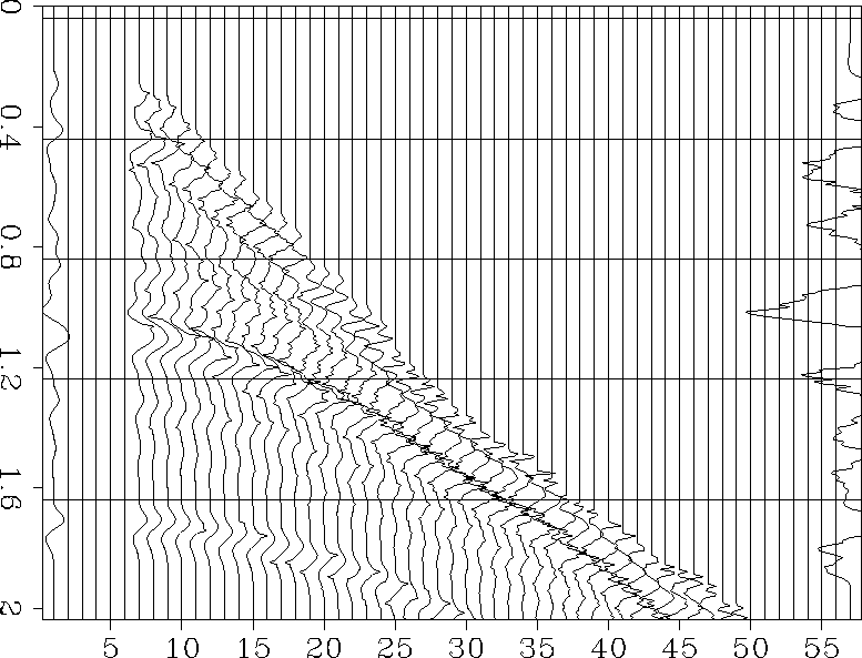
Figure 1 Trace on the left represents the input t(0) model; middle portion is the sprayed, irregularly spaced, CMP gather; right represents the result of applying L followed by L'.
program test use sep ! sep library (for simple I/O) use nnnmo ! generic shift and scale programs use mo_mod ! module containing shift and scale definitions use interpimplicit none real,pointer,dimension(:) :: offset ! trace offsets real,pointer,dimension(:,:) :: in_data,out_data ! cmp values real,pointer,dimension(:) :: velocity ! velocity values real,allocatable,dimension(:) :: t ! x/vel integer :: i2,stat,n1,n2,int real :: o1,d1 ! time axis parameters
call sep_init() ! call from_par("interp",int) ! get interpolation type call from_history (n1,n2) allocate (velocity (n1), offset (n2), in_data (n1,n2), out_data (n1,n2)) call sep_read(velocity,"velocity") ! read in the velocity call sep_read(in_data) ! read in cmp gather call from_history ("o1",o1) call from_history ("d1",d1) call sep_close() call nnnmo_init (o1, o1, d1, n1) ! initiate nmo operator allocate(t(n1)) call sep_read(offset,"offset") ! get offset values do i2=1,n2 ! loop over traces t=offset(i2)/velocity ! init t call nnnmo_step(.true.,int,lin_int,vofz_hyper_time,cos2D_ampl,t) stat=nnnmo_lop(.false.,.false.,in_data(:,i2),out_data (:,i2)) end do call nnnmo_close () ! close nmo operator call sep_write(out_data) ! write out dataset end program test
By performing this `spray' operation (L) followed by its adjoint, NMO (L'), we should recover something close to the input. Figure 1 shows the input trace, the modeled CMP gather, and the result of applying LL'.
 |
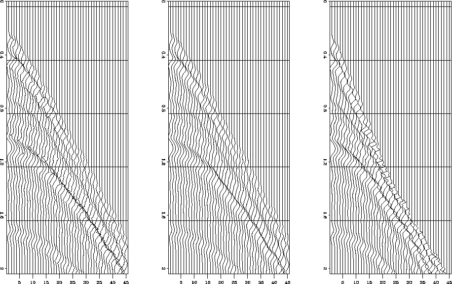
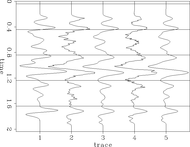
Their are two primary advantages to the object-oriented style. First, it is virtually data independent, no portion of the code makes assumptions on data geometry. Second, because the implementation is highly modular, experimenting with the effect of constant vs. variable velocity, differing interpolation and anti-aliasing schemes, or push vs. pull operator implementation is simple. For example, suppose we wish to see the effect on recovering the original t(0) trace due to variable vs. constant velocity for both linear and nearest-neighbor interpolation. Only the input velocity trace and the interpolation parameter (command-line arguments in the case of simple.f90) need to be altered. Figure 2 shows the resulting CMP gathers while Figure 3 shows the resulting t(0) trace using the different velocity characterizations and interpolation schemes. As expected linear interpolation outperforms nearest-neighbor interpolation in recovering the amplitudes without generating high-frequency noise; also the adjoint is a slightly better approximation when we have constant velocity compared to a v(z) medium.
 |
 |
Rewriting the NMO ``spray and stack'' program for different kinds of transformation (DMO, post-stack and prestack migration, datuming, etc.) becomes a fairly simple exercise.