Numerical Tests

Most of the numerical examples shown below are to demonstrate the advantages of using the spherical, or polar, coordinate system, over the Cartesian one, with this new efficient and unconditionally stable eikonal solver. The Cartesian coordinate implementation includes analytically solving for the first layer of grid points around the point source to reduce the wavefront curvature errors.

At the top of Figure 6, we show the traveltime in a homogeneous medium computed using a second-order in time, or first order in ray parameter, eikonal solver van Trier and Symes (1991), as well as using the grid adaptive scheme to achieve better stability (The code was built by Dave Hale, 1991). This eikonal solver, because of its higher-order accuracy, serves as the reference for testing the accuracy of the fast marching implementation in different coordinate systems. In addition, this particular second-order solver is exact in homogeneous media, because it is executed in polar coordinates. At the bottom of Figure 6, we show the traveltime difference, or error, between implementing the fast-marching method in Cartesian coordinates (left), polar coordinates (right), in contrast to the more accurate second-order scheme. As expected, the majority of the errors in the Cartesian coordinate implementation are concentrated around the 45-degree angle wave propagation. The errors also increase more rapidly near the source where the wavefront curvature is the largest. The polar coordinate implementation, on the other hand, is almost exact for homogeneous media. In this case, the waves propagate in a plane wave geometry with respect to the grid orientation.

 

wkbjvh
Figure 6 The top section shows traveltimes (in seconds) in a homogeneous medium with velocity equal to 2500 m/s, resulting from a source located at the surface at distance 3000 m. The bottom section shows the absolute difference, or errors, in seconds between traveltimes calculated by the fast marching method using the Cartesian coordinates (left) and the polar coordinates (right) in comparison to the more accurate second-order eikonal solver. In this homogeneous case, the polar coordinate fast marching method has practically no errors.

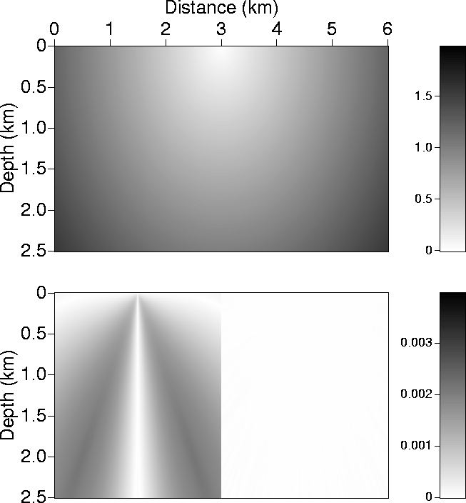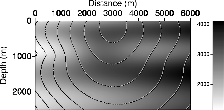
Figure 7 shows traveltimes in a slightly more complicated velocity model. The traveltime contours computed using the various methods practically coincide.

 

vtcont-simpleg
Figure 7 Contours of traveltimes resulting from a source placed on the surface at a distance of 3000 m. The traveltime contours are superimposed on the velocity model (in m/s). The solid black curves correspond to the solution of the more accurate second-order eikonal solver. The gray curves correspond to use of the fast marching eikonal solver in Cartesian coordinates; the dashed curves, in polar coordinates. The three curves are really close.

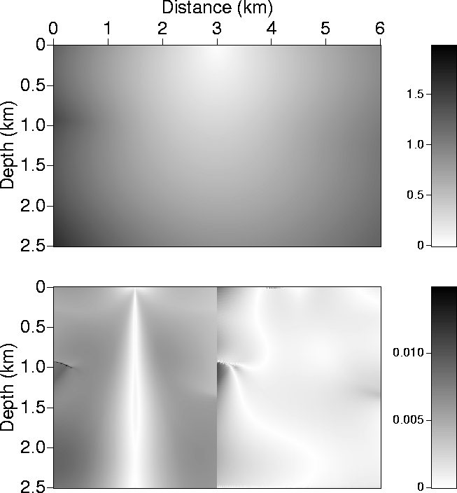
A closer look, in Figure 8, reveals, as in Figure 6, the details of the errors using the different coordinate schemes. The result of using the second-order eikonal solver is shown at the top, and the absolute traveltime errors from using the fast marching method in Cartesian coordinates (left), and polar coordinates (right) are shown at the bottom. The Cartesian and polar coordinate implementations have about the same computational cost; both are far faster than the more accurate second-order scheme. Clearly, the polar coordinate implementation has far fewer errors than the Cartesian coordinate one.

 

wkbjvxz
Figure 8 The top section shows the traveltimes, in seconds, for waves propagating in the model shown in Figure 7, resulting from a source located at the surface at a distance of 3000 m. The bottom sections show the absolute difference, or errors, in seconds between traveltime calculated by the fast marching method using the Cartesian coordinates (left) and the polar coordinates (right) in comparison to the more accurate second-order eikonal solver.