Application to 3-D seismic data regularization

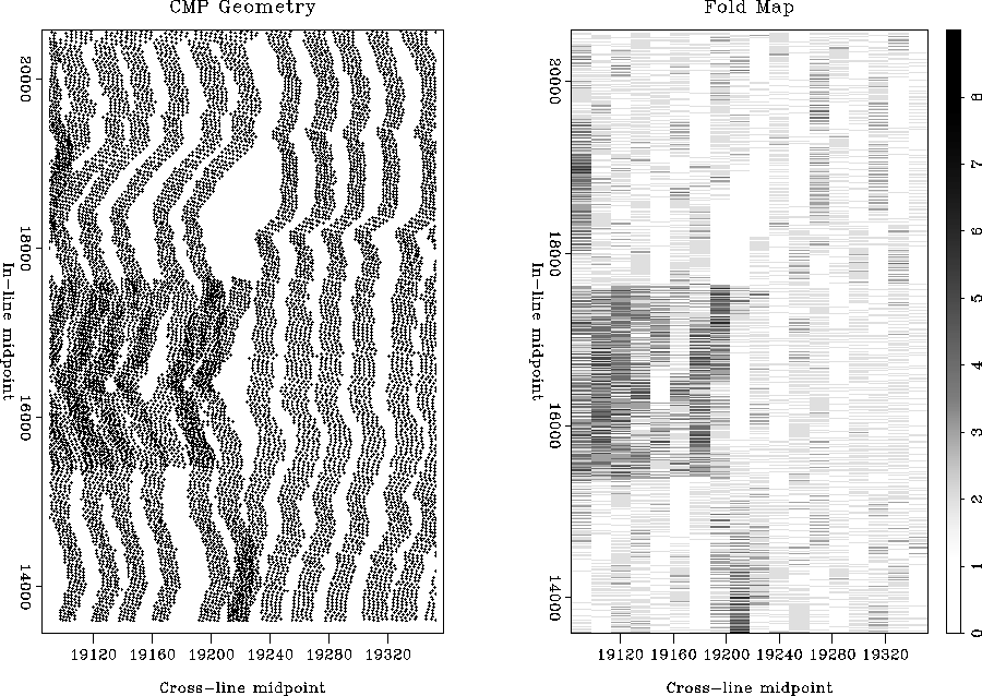
In this subsection, I demonstrate an application of B-spline inverse interpolation for regularizing three-dimensional seismic reflection data. The dataset of this example comes from the North Sea and was used before for testing AMO Biondi et al. (1998) and common-azimuth migration Biondi (1996). Figure  shows the midpoint geometry and the corresponding bin fold for a selected range of offsets and azimuths. The goal of data regularization is to create a regular data cube at the specified bins from the irregular input data, preprocessed by NMO. As typical of marine acquisition, the fold distribution is fairly regular but has occasional gaps caused by the cable feathering effect.

 

cmpfold
Figure 33 Midpoint geometry (left) and fold distribution (right) for the 3-D data test

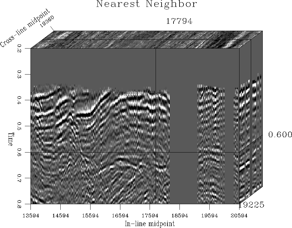
The data cube after normalized binning (inverse nearest neighbor interpolation) is shown in Figure . Binning works reasonably well in the areas of large fold but fails to fill the zero fold gaps and has an overall limited accuracy.

 

bin1
Figure 34 3-D data after normalized binning

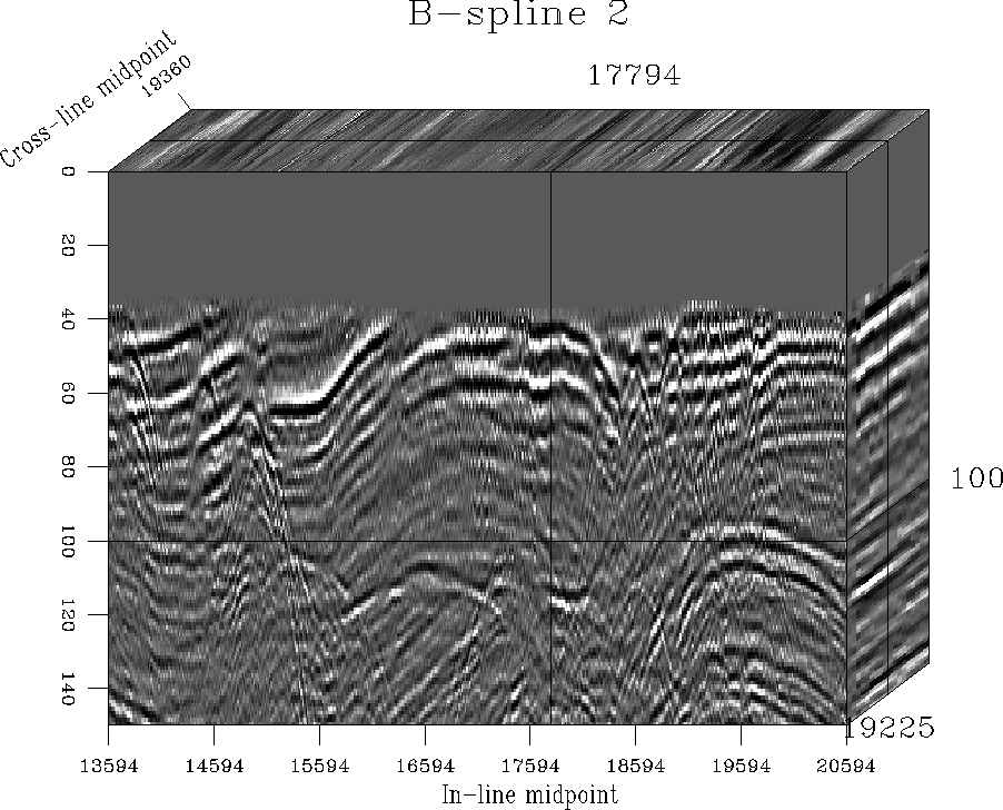
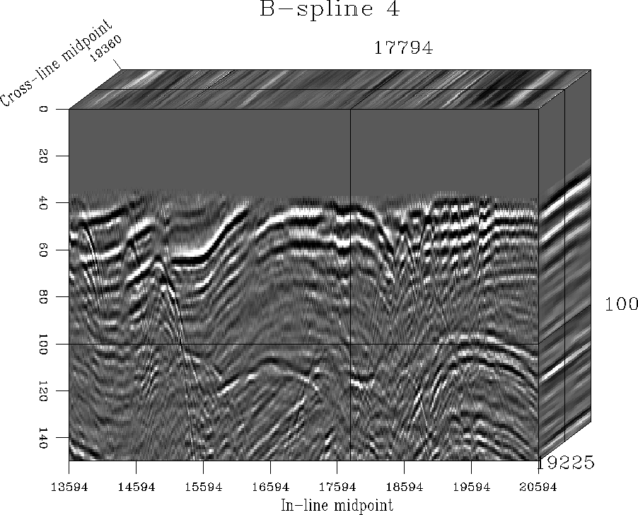
Inverse interpolation using bi-linear interpolants significantly improves the result (Figure ), and inverse B-spline interpolation improves the accuracy even further (Figure ). In both cases, I regularized the data in constant time slices, using recursive filter preconditioning with plane-wave destructor filters analogous to those in Figure . The plane wave slope was estimated from the binned data with the method of Fomel (2000a). The inverse interpolation results preserve both flat reflection events in the data and steeply-dipping diffractions. When data regularization is used as a preprocessing step for common-azimuth migration Biondi and Palacharla (1996), preserving diffractions is important for correct imaging of sharp edges in the subsurface structure.

 

int2
Figure 35 3-D data after inverse interpolation with bi-linear interpolants

 

int4
Figure 36 3-D data after inverse interpolation with third-order B-spline interpolants