Next: Vertical Heterogeneity plus Anisotropy
Up: VERTICAL HETEROGENEITY
Previous: VERTICAL HETEROGENEITY
Nonhyperbolicity of reflection moveout in vertically heterogeneous
isotropic media has been extensively studied with the help of the
Taylor series expansion in the powers of the offset
Al-Chalabi (1973); Bolshykh (1956); Taner and Koehler (1969). The most important property of
vertically heterogeneous media is that the ray parameter  doesn't change with the depth along
each ray (Snell's law). This fact leads to the explicit parametric
relationships
doesn't change with the depth along
each ray (Snell's law). This fact leads to the explicit parametric
relationships
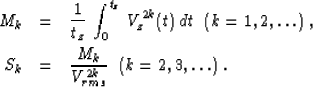
|  |
(23) |
| (24) |
where
|  |
(25) |
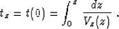
Straightforward differentiation of parametric formulas (23) and
(24) yields the first four coefficients of the Taylor series expansion
|  |
(26) |
in the vicinity of the vertical zero-offset ray. Series (26)
contains only even powers of the offset h because of the reciprocity
principle: the reflection traveltime is an even function of the
offset. Taylor coefficients for the isotropic case are defined as
follows:
| 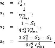 |
(27) |
| (28) |
| (29) |
| (30) |
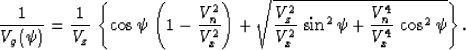
where Vrms2 = M1,
|  |
(31) |
| (32) |
Equation (28) shows that, at small offsets, the reflection moveout
has a hyperbolic form with the normal moveout velocity Vn equal to
the root-mean-square velocity Vrms. At large offsets, however,
the hyperbolic approximation is not accurate. Studying the Taylor
series expansion (26), Malovichko introduced a remarkable
three-parameter approximation for the reflection traveltime in a
vertically heterogeneous isotropic medium
Malovichko (1978); Sword (1987). Malovichko's formula has the form of a
shifted hyperbola Castle (1988); de Bazelaire (1988):
|  |
(33) |
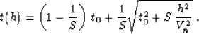
If we set the zero-offset traveltime t0 equal to the vertical
traveltime tz, the velocity Vn equal to Vrms, and the
parameter of heterogeneity S equal to S2, formula
(33) guarantees the correct coefficients a0, a1, and
a2 in the Taylor series (26). Note that the parameter S2
is related to the variance  of the squared velocity
distribution, as follows:
of the squared velocity
distribution, as follows:
|  |
(34) |
According to formula (34), this parameter is always greater
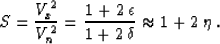
than 1 (it equals 1 in homogeneous media). In the most common
practical cases, the value of S2 lies between 1 and 2. We can
roughly estimate the accuracy of approximation (33) at
large offsets by comparing the fourth term of its Taylor series with
the fourth term of the exact traveltime expansion (26).
According to this estimate, the error of Malovichko's approximation is
| 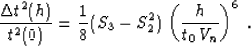 |
(35) |
As follows from the definition of the parameters Sk (32) and
the Schwarz (Cauchy-Bunyakovski) inequality from calculus, expression
(35) is greater than zero for any non-uniform velocity
distribution Vz(tz). This means that Malovichko's approximation
tends to overestimate traveltimes at large offsets. As the offset
approaches infinity, the limit of this approximation is
| 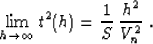 |
(36) |
Formula (36) indicates that the effective horizontal velocity
for Malovichko's approximation (the slope of the shifted hyperbola
asimptote) is different from the normal moveout velocity. We can
interpret this difference as an evidence of the effective
depth-variant anisotropy. However, the anisotropic effect implied in formula
(33) is different from the effect of a homogeneous
transversely isotropic medium described by Thomsen's formula
(1). To reveal this difference, let us substitute the effective
values  ,
,  ,
,  , and
, and  into
(33). After we eliminate the variables z and h, the
resultant expression takes the form
into
(33). After we eliminate the variables z and h, the
resultant expression takes the form
|  |
(37) |
If the anisotropic effect is induced by a vertical heterogeneity,
Vx is greater than Vn, while Vn is greater than Vz. Both of
these inequalities follow from the definitions of Vrms, tv,
and S2 and the Schwartz inequality. They reduce to equalities only
in the case of a constant velocity. Linearizing expression
(37) with respect to Thomsen's anisotropic parameters  and
and  , we can transform it to a form analogous to
that of equation (9), as follows:
, we can transform it to a form analogous to
that of equation (9), as follows:
|  |
(38) |
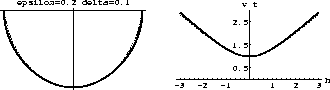
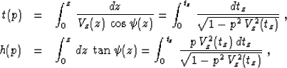
Figure 3 illustrates the difference between the weak
transversally isotropic model and the effective anisotropy implied by
Malovichko's approximation. The difference is noticeable in the shapes
of both the effective wavefront (left plot) and the traveltime curve
(right plot).
nmofrz
Figure 3 Comparing a
weak transversally isotropic model and Malovichko's shifted hyperbola
approximation. The left plot shows effective wavefronts; right:
reflection moveouts. Solid lines correspond to the anisotropic model;
dashed lines: Malovichko's approximation. The values of the effective
vertical, horizontal, and moveout velocities are the same in both
cases and correspond to Thomsen's parameters  ,
,  .
.


Deriving formula (38), we have assumed the correspondence
|  |
(39) |
We could also take the value of the parameter of
heterogeneity S so as to match the coefficient a2 given by formula
(29) with the corresponding term in the Taylor series
(17). In this case, the value of S would be Alkhalifah (1996)
|  |
(40) |
The difference between equations (39) and (40) is an
additional indicator of the fundamental difference between the
homogeneous VTI model and the vertically heterogeneous model. The
three-parameter anisotropic approximation (16) can match the
reflection moveout curve in the isotropic model up to and including
the fourth-order term in the Taylor series expansion, if the value of
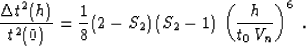
 is chosen in accordance with formula (40). We can
estimate the error of such an approximation with an equation analogous
to (35). It takes the form
is chosen in accordance with formula (40). We can
estimate the error of such an approximation with an equation analogous
to (35). It takes the form
|  |
(41) |
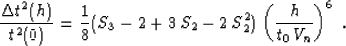
The difference between the error estimates (35) and
(41) is
|  |
(42) |
For the usual values of the parameter of heterogeneity S2, which
range from 1 to 2, expression (42) is greater than
zero. This means that anisotropic approximation (16)
overestimates the traveltimes in the isotropic heterogeneous model
even more than the shifted hyperbola approximation (33)
(as shown in the right plot of Figure 3). Which of the two
approximations is more suitable if the model includes both vertical
heterogeneity and anisotropy? We address this question in the
following subsection.
Next: Vertical Heterogeneity plus Anisotropy
Up: VERTICAL HETEROGENEITY
Previous: VERTICAL HETEROGENEITY
Stanford Exploration Project
9/12/2000