NONSTATIONARITY

Frequencies decrease with time; velocities increase with depth. Reverberation periods change with offset; dips change with location. Still, we often find it convenient to presume that the relevant statistical aspects of data remain constant over a large domain. In mathematical statistics this is called a ``stationarity" assumption. To assume stationarity is to enjoy a simplicity in analysis that has limited applicability in the real world. To avoid seduction by the stationarity assumption we will solve here a problem in which stationarity is obviously an unacceptable presumption. We will gain skill in and feel comfortable with the computer techniques of estimation in moving windows. The first requirement is to learn reliable ways of limiting the potentially destructive effects of the edges of windows.

The way to cope with spatial (or temporal) variation in unknown parameters is to estimate them in moving windows. Formulating the estimation might require special shrewdness so that window edges do not strongly affect the result.

To illustrate computation technique in a nonstationary environment, I have chosen the problem of dip estimation. Before we take up this problem, however, we will examine a generic program for moving a window around on a wall of data. The window-moving operation is so cluttered that the first example of it simply counts the number of windows that hit each point of the wall. Inspecting subroutine nonstat() we first notice that the 1-axis is handled identically with the 2-axis. (Ratfor makes this more obvious than Fortran could.) Notice the bottom of the loops where variables (e1,e2) which will be the ends of the windows are jumped along in steps of (j1,j2). Then notice the tops of the loops where processing terminates when the ends of the windows pass the ends of the wall. Also at the tops of the loops, the window count (k1,k2) is incremented, and the starting points of each window are defined as the window ends (e1,e2) minus their widths (w1,w2).  

# slide a window around on a wall of data.  Count times each data point used.
#
subroutine nonstat( n1,n2, w1,w2, j1,j2, count)
integer n1,n2           # size of data wall
integer w1,w2           # size of window
integer j1,j2           # increments for jumping along the wall
integer s1,s2, e1,e2    # starting and ending points of window on wall
integer k1,k2           # output math size of array of windows
integer i1,i2
real       count( n1,n2)
call null( count, n1*n2)
k2=0; e2=w2; while( e2<=n2) {  k2=k2+1; s2=e2-w2+1
k1=0; e1=w1; while( e1<=n1) {  k1=k1+1; s1=e1-w1+1
        do i1= s1, e1 {
        do i2= s2, e2 {
                count(i1,i2) =  count(i1,i2) + 1.
                }}
        e1=e1+j1            }
        e2=e2+j2            }
return; end

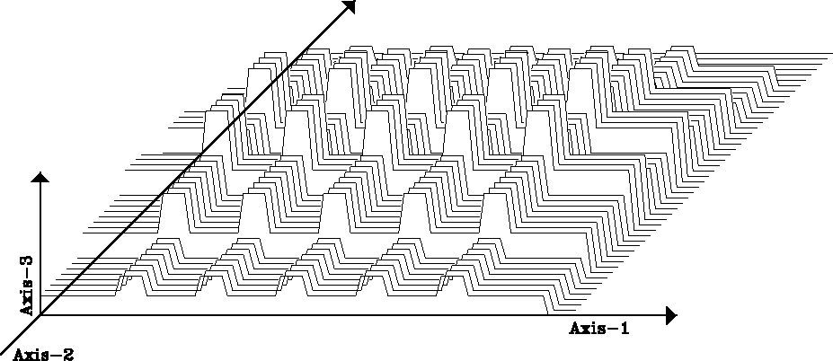
A sample result is shown in Figure 7. Since window widths do not match window jumps, the count is not a constant function of space. We see ridges where the rectangles overlapped a little. Likewise, since the windows were not fitted to the wall, some data values near the end of each axis failed to be used in any window.

 

nonstat Figure 5 Sample output of nonstat() with n1=100, w1=20, j1=15, n2=50, w2=20, j2=8.

Next we address the problem of splicing together data processing outputs derived in each window. This could be done with rectangle weights derived from count in subroutine nonstat() but it is not much more difficult to patch together triangle weighting functions as shown in subroutine nonstat2() .  

# slide a window around on a wall of data.  Triangle weighting.
#
subroutine nonstat2( n1,n2, w1,w2, j1,j2, data, output, weight)
integer              n1,n2, w1,w2, j1,j2,          s1,s2, e1,e2, k1,k2, i1,i2
real    data(n1,n2), output(n1,n2), weight(n1,n2),  triangle1, triangle2, shape
temporary real window(w1,w2), winout(w1,w2)
call null( weight, n1*n2)
call null( output, n1*n2)
k2=0; e2=w2; while( e2<=n2) {  k2=k2+1;  s2=e2-w2+1
k1=0; e1=w1; while( e1<=n1) {  k1=k1+1;  s1=e1-w1+1
        do i1= 1, w1 {
        do i2= 1, w2 {  window(i1,i2) = data(s1+i1-1,s2+i2-1)
                        }}
        do i1= 1, w1 {                          # Trivial data processing
        do i2= 1, w2 {  winout(i1,i2) = window(i1,i2)
                        }}
        do i1= s1, e1 { triangle1= amax1(0., 1. - abs(i1-.5*(e1+s1)) / (.5*w1))
        do i2= s2, e2 { triangle2= amax1(0., 1. - abs(i2-.5*(e2+s2)) / (.5*w2))
                shape = triangle1 * triangle2
                output(i1,i2) = output(i1,i2) + shape * winout(i1-s1+1,i2-s2+1)
                weight(i1,i2) = weight(i1,i2) + shape
                }}
        e1=e1+j1            }
        e2=e2+j2            }
do i1= 1, n1 {
do i2= 1, n2 {  if( weight(i1,i2) > 0. )
                        output(i1,i2) = output(i1,i2) / weight(i1,i2)
        }}
return; end

Triangles allow for a more gradual transition from one window to another. In nonstat2(), data is first pulled from the wall to the window. Next should be the application-specific operation on the data that processes the data window into an output window. (This output is often a residual image of a least squares procedure). To avoid getting into many application-specific details, here we simply copy the input data window to the output window. Next we devise some triangular weighting functions. These are used to weight the output window as it is copied onto the wall of accumulating weighted outputs. Simultaneously, at each point on the wall, the sum of all applied weights is accumulated. Finally, the effect of weight shape and window overlap is compensated for by dividing the value at each point on the wall of outputs by the sum of weights at that point. Figure 7 applies nonstat2() to constant data. As expected, the output is also constant, except at edges where it is zero because no windows overlap the input data. The flattness of the output means that in practice we may allow window overlap greater or less than the triangle half width. Notice that five ridges in Figure 7 correspond to five valleys in Figure 8.

 

nstri
Figure 6 Sample output of nonstat2() with same parameters as Figure 7. Left is weight(n1,n2) and right is output(n1,n2) for constant data. The flattness of the output means that in practice we may allow window overlap greater or less than the triangle half width.

In a typical application, there is one more complication. The filter outputs in each window are shorter than the input data because the filters themselves may not run over the edges else there would be truncation transients. Thus some of the values of the output in each window are undefined. The application-specific filter program may leave these values undefined or it may set them to zero. If they come out zeros, it is safe to add them in to the wall of outputs, but care must be taken that the window weight that is normally accumulated on the wall of weights is omitted. There is one final complication for those of you who plan to be really meticulous. The triangles designed in nonstat2() taper to zero just beyond the ends of the window of data. They should taper to zero just beyond the ends of the window of outputs.