Explicit model for noise

In all the signal analysis above there was no explicit model for noise, but implicitly the idea of noise was there. Now we will recognize it and solve explicitly for it. This leads to what is called ``linear-estimation theory." Instead of simply Y=FX, we add noise $N(\omega)$into the defining equation:  

$$Y(\omega) \eq F(\omega)X(\omega) + N(\omega)$$ (19)

To proceed we need to define the ``variance" (described more fully in chapter ) as  

$$\sigma_X^2 \eq {1\over n} \ \sum_{j=1}^n \bar X(\omega_j)X(\omega_j)$$ (20)

and likewise the noise variance $\sigma_N^2$.

The general linear-estimation method minimizes something that looks like a sum of relative errors:  

$$Q(X,N) \eq { \bar X\,X \over \sigma_X^2 } \ +\ { \bar N\,N \over \sigma_N^2 }$$ (21)

Notice that the variances put both terms of the sum into the same physical units. I have not derived equation (21) but stated it as reasonable: from it we will derive reasonable answers which we have already seen. The rationale for the minimization of (21) is that we want the noise to be small, but because we must guard against zero division in X=Y/F, we ask for X to be small too. Actually, by introducing equation (19), we have abandoned the model X=Y/F and replaced it with the model X=(Y-N)/F. Thus, instead of thinking of falsifying F to avoid dividing by zero in X=Y/F, we now think of finding N so the numerator in (Y-N)/X vanishes wherever the denominator does.

By introducing (19) into (21) we can eliminate either N or X. Eliminating N, we have  

$$Q(X) \eq { \bar X\,X \over \sigma_X^2 } \ +\ { (\overline{FX-Y})(FX-Y) \over \sigma_N^2 }$$ (22)

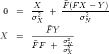
Minimizing Q(X) by setting its derivative by $\bar X$ to zero gives

$$\begin{eqnarray} 0 &=& {X \over \sigma_X^2} \ +\ {\bar F(FX-Y)\over \sigma_N^2} \ X &=& {\bar F Y \over \bar F F \ +\ {\sigma_N^2 \over \sigma_X^2}}\end{eqnarray}$$ (23) (24)

Equation (24) is the same as equation (12), except that it gives us a numerical interpretation of the value of $\epsilon$ in equation (12).

We can find an explicit equation for the noise in terms of the data and filter by substituting equation (24) into equation (19) and solving for N.