 |
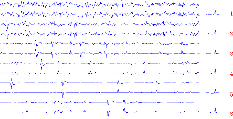
Figure 14 Four independent trials of deconvolution of sparse noise into an all-pass filter. Alternate lines are input and output.
If we carefully examine the analysis leading to that conclusion, we will find lurking the assumption that the weighting function used in the least-squares estimation is uniform. And when this assumption is wrong, so is our conclusion, as Figure 14 shows.
 |
Recall that the inverse to an all-pass filter is its time reverse. The reversed shape of the filter is seen on the inputs where there happen to be isolated spikes.
Let us see what theory predicts cannot be done, and then I will tell you how I did it. If you examine the unweighted least-squares error-filter programs, you will notice that the first calculation is the convolution operator and then its transpose. This takes the autocorrelation of the input and uses it as a gradient search direction. Take a white input and pass it through a phase-shift filter; the output autocorrelation is an impulse function. This function vanishes everywhere except for the impulse itself, which is constrained against rescaling. Thus the effective gradient is zero. The solution, an impulse filter, is already at hand, so a phase-shift filter seems unfindable.
On the other hand, if the signal strength of the input varies,
we should be balancing its expectation by weighting functions.
This is what I did in Figure 14.
I chose a weighting function equal to the inverse of the absolute value
of the output of the filter plus an ![]() .Since the weighting function depends on the output,
the process is iterative.
The value of
.Since the weighting function depends on the output,
the process is iterative.
The value of ![]() chosen was 20% of the maximum signal value.
chosen was 20% of the maximum signal value.
Since the iteration is a nonlinear procedure, it might not always work. A well-established body of theory says it will not work with Gaussian signals, and Figure 15 is consistent with that theory.
 |
In Figure 13, I used weighting functions roughly inverse to the envelope of the signal, taking a floor for the envelope at 20% of the signal maximum. Since weighting functions were used, the filters need not have turned out to be symmetrical about their centers, but the resulting asymmetry seems to be small.