The slow FT code

The slowft() routine exhibits features found in many physics and engineering programs. For example, the time-domain signal (which I call ``tt()"), has nt values subscripted, from tt(1) to tt(nt). The first value of this signal tt(1) is located in real physical time at t0. The time interval between values is dt. The value of tt(it) is at time t0+(it-1)*dt. I do not use ``if'' as a pointer on the frequency axis because if is a keyword in most programming languages. Instead, I count along the frequency axis with a variable named ie. 

subroutine slowft( adj, add, nyq, t0,dt,nt,tt,  f0,df,  nf,ff)
integer it,ie,     adj, add, nyq,       nt,                nf
complex cexp, cmplx,                    tt(nt),         ff(nf)
real pi2, freq, time, scale,       t0,dt,        f0,df
call adjnull(      adj, add,            tt,2*nt,        ff,2*nf)
                        pi2= 2. * 3.14159265;           scale = 1./sqrt( 1.*nt)
                        df = (1./dt) / nf
                if( nyq>0)
                        f0 =   - .5/dt  
                else
                        f0 =   - .5/dt + df/2.
do ie = 1, nf {   freq= f0 + df*(ie-1)
do it = 1, nt {   time= t0 + dt*(it-1)
        if( adj == 0 )
                ff(ie)= ff(ie) + tt(it) * cexp(cmplx(0., pi2*freq*time)) * scale
        else
                tt(it)= tt(it) + ff(ie) * cexp(cmplx(0.,-pi2*freq*time)) * scale
        }}
return; end

The total frequency band is $2\pi$ radians per sample unit or $1/\Delta t$ Hz. Dividing the total interval by the number of points nf gives $\Delta f$.We could choose the frequencies to run from 0 to $2\pi$ radians/sample. That would work well for many applications, but it would be a nuisance for applications such as differentiation in the frequency domain, which require multiplication by $-i\omega$including the negative frequencies as well as the positive. So it seems more natural to begin at the most negative frequency and step forward to the most positive frequency. Next, we must make a confusing choice.

Refer to Figure 1. We could begin the frequency axis at the negative Nyquist, $-.5/\Delta t$ Hz; then we would finish one point short of the positive Nyquist. This is shown on the left two circles in Figure 1. Alternately, for the right two circles we could shift by half a mesh interval, so the points would straddle the Nyquist frequency. To do this, the most negative frequency would have to be $-.5/{\Delta t}+\Delta f /2$ Hz. In routine slowft() and in the test results, ``nyq=1'' is a logical statement that the Nyquist frequency is in the dataset. Oppositely, if the Nyquist frequency is interlaced by the given frequencies, then nyq=0. Finally, the heart of the program is to compute either a Fourier sum, or its inverse, which uses the complex conjugate.

The routine ftlagslow() below simply transforms a signal to the Fourier domain, multiplies by $\exp( i \omega t_0)$, where t₀ is some desired time lag, and then inverse transforms to the time domain. Notice that if the negative Nyquist frequency is present, it is treated as the average of the negative and positive Nyquist frequencies. If we do not take special care to do this, we will be disappointed to find that the time derivative of a real-time function develops an imaginary part.

 

subroutine ftlagslow( nyq, lag, t0,dt, n1, ctt)
integer nyq, n1, ie
real lag, t0, dt, f0, df, freq
complex ctt(n1), cexp, cmplx
temporary complex cff(n1)

call slowft( 0, 0, nyq, t0, dt, n1, ctt, f0, df, n1, cff)

do ie= 1, n1 {  freq= f0 + (ie-1)*df
        if( ie==1  &&  nyq > 0)
                cff(1)  = cff(1)  * cos(            2.*3.14159265 * freq * lag )
        else
                cff(ie) = cff(ie) * cexp( cmplx(0., 2.*3.14159265 * freq * lag))
        }
call slowft( 1, 0, nyq, t0, dt, n1, ctt, f0, df, n1, cff)

return; end

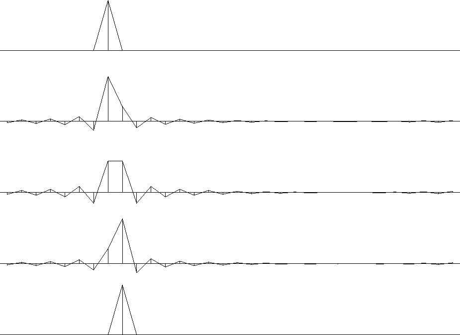
Figure 4 shows what happens when an impulse is shifted by various fractions of a sample unit with subroutine ftlagslow(). Notice that during the delay, the edges of the signals ripple--this is sometimes called the ``Gibbs ripple.'' You might find these ripples annoying, but it is not easy to try to represent an impulse halfway between two mesh points. You might think of doing so with (.5,.5), but that lacks the high frequencies of an ideal impulse.

 

delay Figure 3 An impulse function delayed various fractions of a mesh point. Pushbutton for interaction (experimental).

The routine ftderivslow() below is the Fourier-domain routine for computing a time derivative by multiplying in the frequency domain by $-i\omega$. 

subroutine ftderivslow( nyq, t0,dt, ntf, ctt, cdd)
integer nyq, ntf, ie
real t0,dt,f0,df, freq
complex ctt(ntf), cdd(ntf), cmplx
temporary complex cff(ntf)
call slowft( 0, 0, nyq, t0, dt, ntf, ctt, f0, df, ntf, cff)

do ie= 1, ntf {  freq= f0+(ie-1)*df
        cff(ie) = cff(ie) *  cmplx( 0., - 2. * 3.141549265 * freq )
        }
if( nyq > 0 )                                           #  if( omega0 == -pi/dt)
        cff(1) = 0.

call slowft( 1, 0, nyq, t0, dt, ntf, cdd, f0, df, ntf, cff)
return; end