Convolution end effects

In practice, filtering generally consists of three parts: (1) convolution, (2) shifting to some preferred time alignment, and (3) truncating so the output has the same length as the input. An adjoint program for this task, is easily built from an earlier program. We first make a simple time-shift program advance(). 

# signal advance:    y(iy) = x(iy+jump)
#
subroutine advance( adj, add, jump, nx, xx, ny, yy)
integer ix, iy,     adj, add, jump, nx,     ny
real                                    xx(nx), yy(ny)
call adjnull( adj, add,                 xx,nx,  yy,ny)
do iy= 1, ny {
        ix = iy + jump
        if(         ix >= 1 )
                if( ix <= nx )
                        if( adj == 0 )
                                yy( iy) = yy( iy) + xx( ix)
                        else
                                xx( ix) = xx( ix) + yy( iy)
        }
return; end

Although the code is bulky for such a trivial program, it is easy to read, works for any size of array, and works whether the shift is positive or negative. Since filtering ordinarily delays, the advance() routine generally compensates.

Merging advance() with the earlier program contran() according to the transpose rule $(\bold A \bold B)' = \bold B' \bold A'$,we get contrunc().  

#       Convolve, shift, and truncate output.
#
subroutine contrunc( conj, add, lag,  np,pp,  nf,ff,  nq,qq)
integer ns,          conj, add, lag,  np,     nf,     nq
real    pp(np)                          # input data
real    ff(nf)                          # filter (output at ff(lag))
real    qq(nq)                          # filtered data
temporary real ss( np+nf-1)
ns = np + nf - 1
if( conj == 0 ) {
        call contran( 0, 0, np,pp, nf,ff, ss)
                                call advance( 0, add, lag-1, ns,ss, nq,qq)
        }
else {                          call advance( 1,   0, lag-1, ns,ss, nq,qq)
        call contran( 1, add, np,pp, nf,ff, ss)
        }
return; end

For a symmetrical filter, a lag parameter half of the filter length would be specified. The output of a minimum-phase filter is defined to be at the beginning of the filter, ff(1), so then lag=1. The need for an adjoint filtering program will be apparent later, when we design filters for prediction and interpolation. The program variable add happens to be useful when there are many signals. Our first real use of add will be found in the subroutine stack1() .

Another goal of convolution programs is that zero data not be assumed beyond the interval for which the data is given. This can be important in filter design and spectral estimation, when we do not want the truncation at the end of the data to have an effect. Thus the output data is shorter than the input signal. To meet this goal, I prepared subroutine convin(). 

#       Convolve and correlate with no assumptions off end of data.
#
subroutine convin( adj, add, nx, xx, nb, bb, yy)
integer ib, iy,ny, adj, add, nx,     nb
real    xx(nx)                  # input signal
real    bb(nb)                  # filter      (or output crosscorrelation)
real    yy(nx-nb+1)             # filtered signal (or second input signal)
ny = nx - nb + 1                # length of filtered signal
if( ny < 1 )  call erexit('convin() filter output negative length.')
call adjnull(      adj, add,         bb, nb, yy, ny)
if( adj == 0 )
        do iy= 1, ny {
        do ib= 1, nb {
                        yy( iy) = yy( iy) + bb(ib) * xx( iy-ib+nb)
                        }}
else
        do ib= 1, nb {
        do iy= 1, ny {
                        bb( ib) = bb( ib) + yy(iy) * xx( iy-ib+nb)
                        }}
return; end

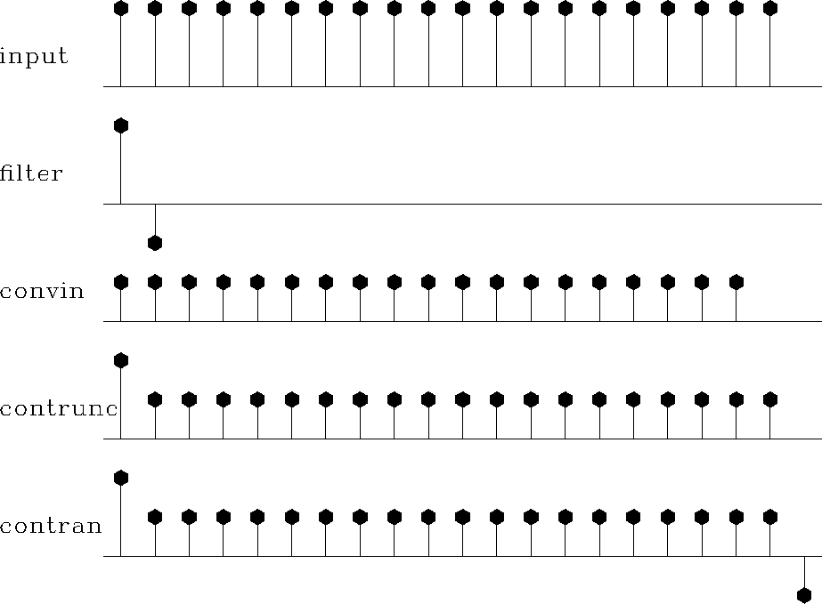
By now you are probably tired of looking at so many variations on convolution; but convolution is the computational equivalent of ordinary differential equations, its applications are vast, and end effects are important. The end effects of the convolution programs are summarized in Figure 1.

 

conv Figure 1 Example of convolution end effects. From top to bottom: (1) input; (2) filter; (3) output of convin(); (4) output of contrunc() with no lag (lag=1); and (5) output of contran().