Noise, surface waves and clip

If seismic data contained nothing but reflections, then there would be little trouble plotting it. You would simply multiply by t² and then scale so that the largest data values stayed in the available plotting area. In reality there are two problems: (1) noisy traces and (2) noise propagation modes. We have noisy traces because the people in the world won't all be quiet while we listen for echoes. Noise propagation modes are waves trapped in surface layers. So their divergence is in a two-dimensional space rather than the three-dimensional space for reflections. Water noises are additionally strong because of the homogeneity and low absorption of water.

Noises are handled by ``clipping'' data values at some level lower than the maximum. Clipping means that values larger than the clip value are replaced by the clip value. Since the size of the noise is generally unpredictable, the most reliable method is to use quantiles. Imagine the data points sorted in numerical order by the size of their absolute values. The $n^{ {\rm th}}$ quantile is defined as the absolute value that is n/100 of the way between the smallest and largest absolute value. So if data is clipped at the $99^{{{\rm }} th}$ percentile, then up to one percent of the data can be infinitely strong noise. I find that most field profiles have less than 10% noisy points. So I often clip at thrice the $90^{ {\rm th}}$ percentile. To find the quantile, it is not necessary to fully sort the data. That would be slow. Hoare's algorithm is much faster (see FGDP or Claerbout and Muir [1973] for full reference and more geophysical context).

Different plots have different purposes. It is often important to preserve linearity during processing, but at the last stage--plotting--linearity can be sacrificed to enable us to see all events, large and small. After all, human perceptions are generally logarithmic. In our lab we generally use power laws. I find that replacing data points by their signed square roots generally compresses all signals into a visible range. When plotting field profiles with a very close trace spacing, it may be better to use the signed cube roots. More generally, we do non-linear gain with  

$$\hbox{Display} \eq \sgn ( \hbox{Data} ) \ \ \vert \hbox{Data} \vert^{\gamma}$$ (1)

Gamma is a term in photography to describe nonlinearity of photographic film. Most of the data plots in this book use $\gamma =1$, t² gain, and clip at the $99^{{{\rm }} th}$ percentile.

The industry standard approach seems to be AGC (Automatic Gain Control). AGC means to average the data magnitude in some interval and then divide by the magnitude. Although AGC is nonlinear, it is more linear than using $\gamma$ so it is presumably better if you plan later processing. But with AGC, you lose reversibility and the sense of absolute gain.

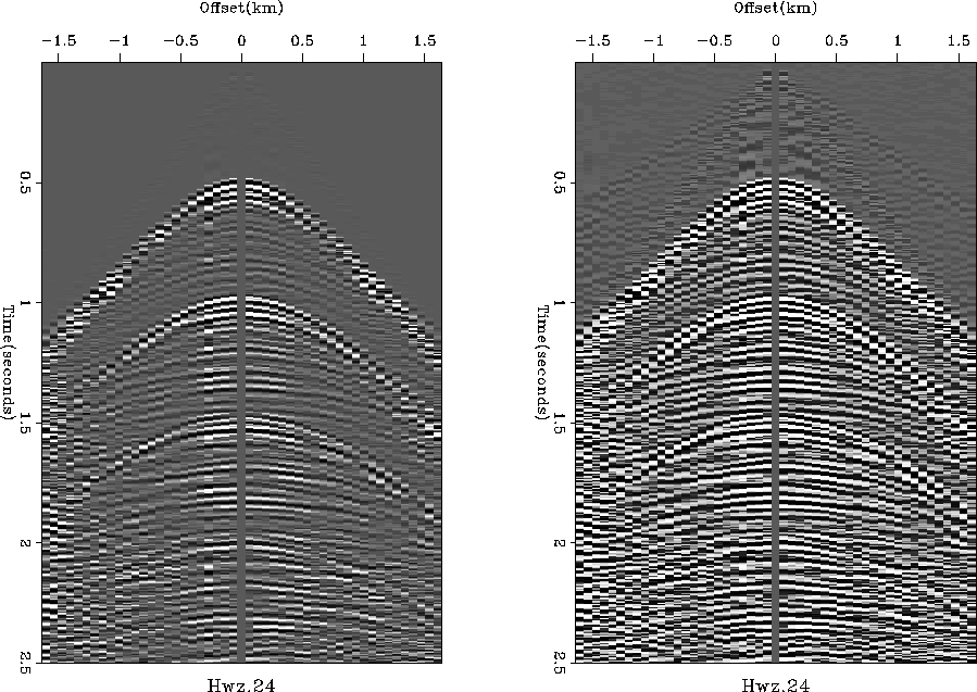
Figure 2 is an interesting example.

 

arctic
Figure 2 Arctic profile from Western Geophysical. Left, with t². Center with t² and $\gamma =0.4$. Right, with Western's AGC.

Since it is a split spread, you assume it to be land data. Ships can't push cables in front of them. But the left panel clearly shows marine multiples. The reverberation period is uniform, and there are no reflections before the water bottom. It must be data collected on ice over deep water (375m). From the non-linear gain in the center panel we clearly see a water wave, and before it a fast wave in the ice. There is also weak low-velocity, low-frequency ``ground roll'' on the ice. There are also some good reflections.