Since velocity increases with depth,
at wide enough offset a deep enough path
will arrive sooner than a shallow path.
In other words,
traveltime curves for shallow events
must cut across the curves of deeper events.
Where traveltime curves cross,
NMO is no longer a one-to-one transformation.
To see what happens to the stacking process
I prepared Figures 3-5
using a typical marine recording geometry
(although for clarity I used
larger ![]() ) and we will use
a typical Texas gulf coast average velocity,
) and we will use
a typical Texas gulf coast average velocity,
![]() where
where ![]() .
.
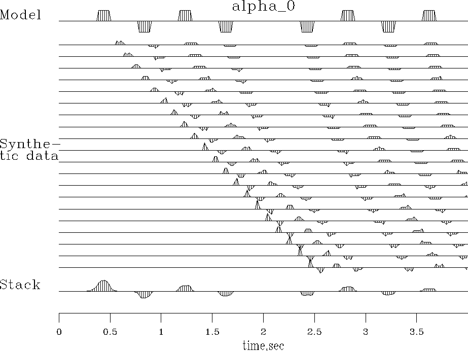
First we repeat the calculation of Figure 2
with constant velocity ![]() and more reflectors.
We see in Figure 3 that the stack reconstructs
the model except for two details:
(1) the amplitude diminishes with time, and
(2) the early waveforms have become rounded.
and more reflectors.
We see in Figure 3 that the stack reconstructs
the model except for two details:
(1) the amplitude diminishes with time, and
(2) the early waveforms have become rounded.
|
nmo0alfa0
Figure 3 Synthetic CMP gather for constant velocity earth and reconstruction. |  |
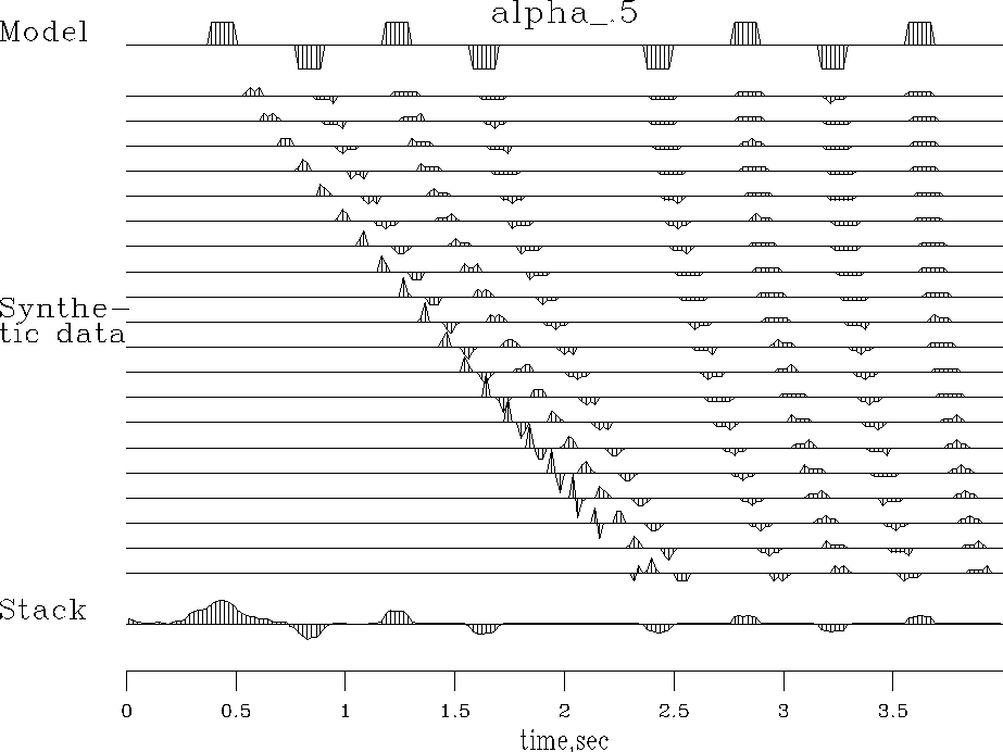
Then we repeat the calculation
with the Gulf coast typical velocity gradient ![]() .The polarity reversal on the first arrival of the wide offset trace
in Figure 4
is evidence that in practice traveltime curves do cross.
(As was plainly evident in Figures
.The polarity reversal on the first arrival of the wide offset trace
in Figure 4
is evidence that in practice traveltime curves do cross.
(As was plainly evident in Figures
![[*]](http://sepwww.stanford.edu/latex2html/cross_ref_motif.gif) ,
,
![[*]](http://sepwww.stanford.edu/latex2html/cross_ref_motif.gif) and
and
![[*]](http://sepwww.stanford.edu/latex2html/cross_ref_motif.gif) crossing traveltime curves are even more significant elsewhere in the world.)
Comparing Figure 3 to Figure 4
we see that an effect of the velocity gradient
is to degrade the stack's reconstruction of the model.
Velocity gradient has ruined the waveform on the shallowest event,
at about 400ms.
If the plot were made on a finer mesh
with higher frequencies,
we could expect ruined waveforms a little deeper too.
crossing traveltime curves are even more significant elsewhere in the world.)
Comparing Figure 3 to Figure 4
we see that an effect of the velocity gradient
is to degrade the stack's reconstruction of the model.
Velocity gradient has ruined the waveform on the shallowest event,
at about 400ms.
If the plot were made on a finer mesh
with higher frequencies,
we could expect ruined waveforms a little deeper too.
|
nmo0alfa.5
Figure 4 Synthetic CMP gather for velocity linearly increasing with depth (typical of Gulf of Mexico) and reconstruction. |  |
Our NMO and stack subroutines can be used for modeling or for data processing.
In designing these programs we gave no thought to signal amplitudes
(although results showed an interesting AVO effect in Figure 2.)
We could redesign the programs so that the modeling operator has the
most realistic amplitude that we can devise.
Alternately, we could design the amplitudes
to get the best approximation to
![]() which should result in ``Stack''
being a good approximation to ``Model.''
I experimented with various weighting functions until
I came up with
subroutines nmo1()
which should result in ``Stack''
being a good approximation to ``Model.''
I experimented with various weighting functions until
I came up with
subroutines nmo1() ![[*]](http://sepwww.stanford.edu/latex2html/cross_ref_motif.gif) and stack1() (like stack0()
and stack1() (like stack0() ![[*]](http://sepwww.stanford.edu/latex2html/cross_ref_motif.gif) )
which embodies the weighting function
)
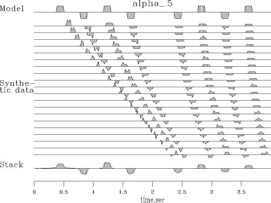
which embodies the weighting function ![]() and which produces the result in Figure 5.
and which produces the result in Figure 5.
|
nmo1alfa.5
Figure 5 Synthetic CMP gather for velocity linearly increasing with depth and reconstruction with weighting functions in subroutine nmo1(). Lots of adjustable parameters here. |  |
The result in Figure 5 is very pleasing.
Not only is the amplitude as a function of time better preserved,
more importantly, the shallow wavelets are less smeared
and have recovered their rectangular shape.
The reason the reconstruction is much better is
the cosine weighting implicit in ![]() .It has muted away much of the energy in the shallow asymptote.
I think this energy near the asymptote is harmful
because the waveform stretch is so large there.
Perhaps a similar good result could be found by experimenting
with muting programs such as mutter()
.It has muted away much of the energy in the shallow asymptote.
I think this energy near the asymptote is harmful
because the waveform stretch is so large there.
Perhaps a similar good result could be found by experimenting
with muting programs such as mutter() ![[*]](http://sepwww.stanford.edu/latex2html/cross_ref_motif.gif) .
However, subroutine nmo1()
.
However, subroutine nmo1() ![[*]](http://sepwww.stanford.edu/latex2html/cross_ref_motif.gif) differs from mutter()
in two significant respects:
(1) nmo1() is based on a theoretical concept
whereas mutter() requires observational parameters
and (2) mutter() applies a weighting in
the coordinates of the (t,x) input space,
while nmo1() does that
but also includes the coordinate
differs from mutter()
in two significant respects:
(1) nmo1() is based on a theoretical concept
whereas mutter() requires observational parameters
and (2) mutter() applies a weighting in
the coordinates of the (t,x) input space,
while nmo1() does that
but also includes the coordinate ![]() of the the output space.
With nmo1() events from different
of the the output space.
With nmo1() events from different ![]() depths see different mutes
which is good where a shallow event asymptote
crosses a deeper event far from its own asymptote.
In practice the problem of crossing traveltime curves is severe,
as evidenced by
Figures
depths see different mutes
which is good where a shallow event asymptote
crosses a deeper event far from its own asymptote.
In practice the problem of crossing traveltime curves is severe,
as evidenced by
Figures ![[*]](http://sepwww.stanford.edu/latex2html/cross_ref_motif.gif) -
-![[*]](http://sepwww.stanford.edu/latex2html/cross_ref_motif.gif) and both weighting during NMO and muting should be used.
and both weighting during NMO and muting should be used.
subroutine nmo1( adj, add, slow,    x, t0, dt, n,zz,  tt )
integer  it, iz, adj, add,                        n
real  xs, t , z,           slow(n), x, t0, dt, zz(n), tt(n), wt
call adjnull(    adj, add,                     zz,n,  tt,n)
do iz= 1, n {   z = t0 + dt*(iz-1)
                xs = x * slow(iz)
                t = sqrt ( z * z + xs * xs) + 1.e-20
                wt = z/t * (1./sqrt(t))                 #  weighting function
                it = 1 + .5 + (t - t0) / dt
                if( it <= n )
                        if( adj == 0 )
                                tt(it) = tt(it) + zz(iz) * wt
                        else
                                zz(iz) = zz(iz) + tt(it) * wt
           }
return; end
It is important to realize that the most accurate possible
physical amplitudes are not necessarily those for which
![]() .Physically accurate amplitudes involve many theoretical
issues not covered here.
It is easy to include some effects
(spherical divergence based on velocity depth variation)
and harder to include others
(surface ghosts and arrays).
We omit detailed modeling here
because it is the topic of so many other studies.
.Physically accurate amplitudes involve many theoretical
issues not covered here.
It is easy to include some effects
(spherical divergence based on velocity depth variation)
and harder to include others
(surface ghosts and arrays).
We omit detailed modeling here
because it is the topic of so many other studies.