Impulse response

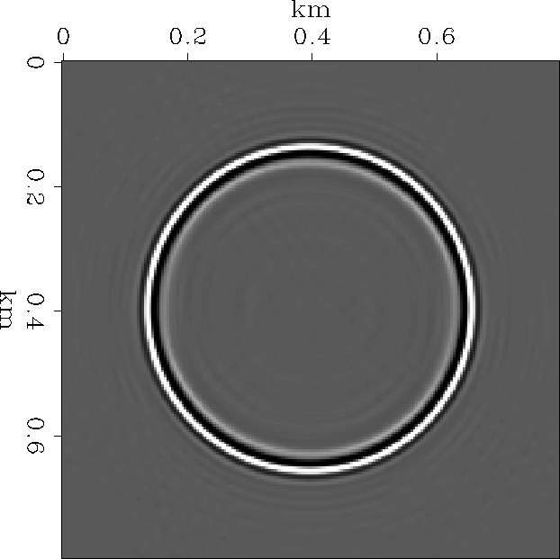
A slice through the broad-band impulse response of the 45$^\circ$equation is shown in Figure 1. As with the 2-D implementation of the 45$^\circ$ equation, evanescent energy at high dip appears as noise, and takes the form of a cardioid. This is never a problem on field data, and has been removed from the depth-slice shown in Figure 2. Implicit migration with the full Laplacian, instead of a splitting approximation, produces an impulse response that is azimuthally isotropic without the need for any phase corrections.

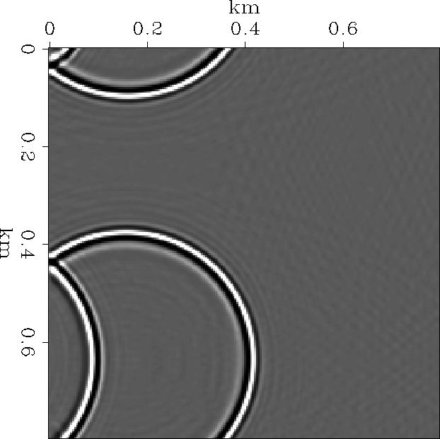
Figure 3 shows the effects of the different boundary conditions on the two spatial axes. The fast spatial axis (top and bottom of Figure) have helical boundary conditions, and show wrap-around. The slow spatial axis (left and right of Figure) has a zero-value boundary condition, and hence is reflective.

For the examples in this paper, we set the `one-sixth' parameter Claerbout (1985), $\beta_{1/6}=0.125$, and used the isotropic nine-point Laplacian from equation (8).

 

3Dtimeslice Figure 2 Depth-slice of centered impulse response corresponding to a dip of 45$^\circ$. Note the azimuthally isotropic nature of the full implicit migration. Evanescent energy has been removed by dip-filtering prior to migration.

 

3Dboundary Figure 3 Depth-slice of offset impulse response corresponding to a dip of 45$^\circ$. Note the helical boundary conditions on the fast spatial axis.