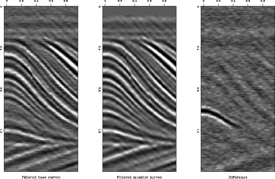
Instead of taking the minimum of the two surveys, as in equation (3), I took the lower value if it was below some threshold, B1, and the higher value if it was greater than another threshold, B2. For values in between I took a scaled linear combination:
| (7) |
For the example shown in Figure 6,
I used ![]() and
and ![]() of
of ![]() . The
bandwidth equalization was done in the frequency domain and the phase
matching in the time domain.
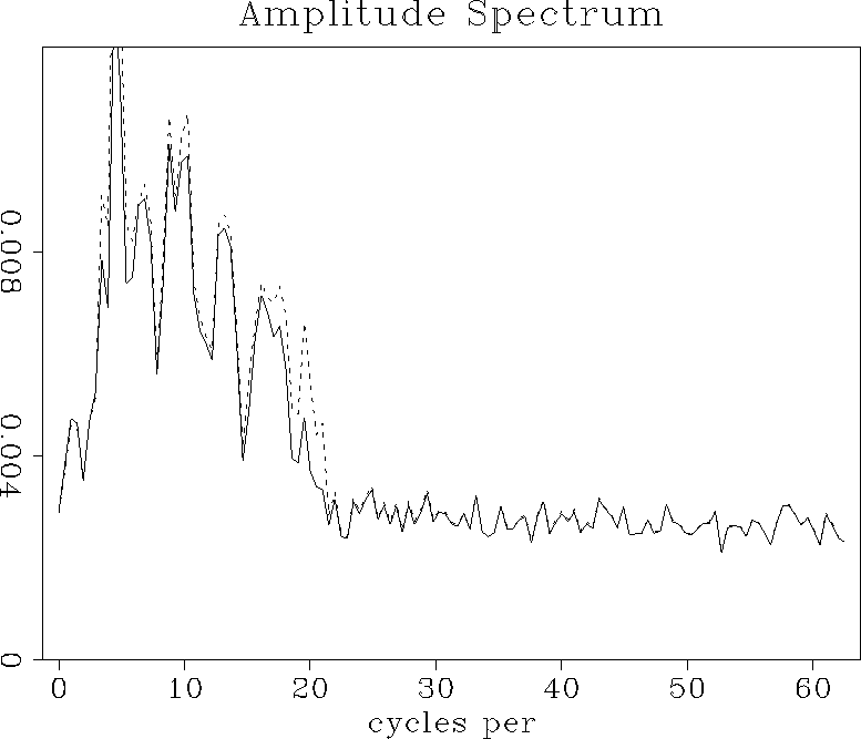
Figure 7 shows the
spectra of the difference sections for this approach and the standard
mixed domain approach. The bandwidth has been increased by a small
amount, while the noise level has remained constant, so this approach
has worked to a small extent.
. The
bandwidth equalization was done in the frequency domain and the phase
matching in the time domain.
Figure 7 shows the
spectra of the difference sections for this approach and the standard
mixed domain approach. The bandwidth has been increased by a small
amount, while the noise level has remained constant, so this approach
has worked to a small extent.
 |
|
opt.spec
Figure 7 Spectra of difference plots. Solid line is standard mixed domain approach, and dashed line is `optimal' mixed domain approach. |  |