Building and interpreting the depth error panel

The focusing principles can be understood by thinking of a point diffractor. The seismic response of a point diffractor is an hyperboloid in 3-D or an hyperbola in 2-D (Z=0). If a CMP gather is downward continued with the real propagation velocity (V_m=V_r) to the real point diffractor depth, z_r (imaging condition: t=0s), the diffracted energy is collapsed to the hyperbola apex and the energy is maximum. The point diffractor position (x_m,y_m,Z_m) is equal to the point diffractor point at (x_r,y_r,z_r) (see Figure 1). If the velocity is changed ($V_{m} \neq V_{r}$) and the CMP is downward continued, the image obtained at the imaging condition (t=0 s) is not well focused and its energy is not maximum at the hyperbola apex. For this new velocity, there is a focusing point, where the energy is maximum at the zero-offset trace, but its spatial position and depth differ from the real position.

Based on the work of Doherty and Claerbout (1974) and MacKay and Abma (1992), the focusing point depth Z_f obtained with migration velocity is equal to the real depth Z_r if the migration velocity is equal to the real propagation velocity V_r:  

$$2\frac{Z_{r}}{V_{r}} = 2\frac{Z_{m}}{V_{m}}.$$ (2)

Equation (2) is valid on the imaging line (t=0 s) (see Figure 2) and is still valid for velocities V_m close to V_r. Replacing V_m in equation (1), the real depth is expressed as function of the focusing depth:  

$$Z_{r}=\sqrt{Z_{m}Z_{f}} \equiv \frac{Z_{m}+Z_{f}}{2},$$ (3)

The vertical depth error is defined by  

$$\delta = \frac{Z_{f}-Z_{m}}{2},$$ (4)

where Z_f is estimated from the error depth gather defined by the zero-offset trace chosen at every downward continued operator step. Moreover, the depth error formula (Equation (4)) is used to define the depth error gather. It is important to remember that focusing analysis is a technique for making estimations of the real RMS velocity V_r.

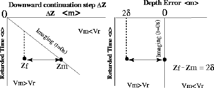
Figure 1 shows the focusing panel and depth error panel. A long the x-axes of the focusing panel is plotted the downward continuation step, where every zero-offset trace is chosen. In the vertical axis is the retarded time ${\tau}$ defined by the recording time, and the vertical time to the current downward continuation step, divided by the velocity V_m:  

$$\tau=t + \frac{2Z}{V_{m}}.$$ (5)

On the diagonal of the focusing panel equation (2) is defined and is the imaging line where the focusing energy is located when the CMP data is downward continued with the real propagation velocity (i.e., V_m=V_r).

Using the focusing panel and applying the lateral shift defined by the equation (4), the depth error panel is built. Now, the imaging line is the zero error line and the vertical axes is the retarded time. Working with the retarded time allows us to compensate the time shifting between traces of different downward continuation steps Claerbout (1984).

In heterogeneous media focusing analysis fails due to the assumption that the Z_m, Z_r and Z_f are aligned along the same ray path (see Figure 3). To solve this problem Audebert and Diet (1993) suggests correcting the depth focusing panel by residual zero-offset migration with the migration velocity, to obtain a depth focusing panel in agreement with normal incidence ray (in the horizontal layered media it is a vertical path, (see Figure 2). Jeannot and Berranger (1994) suggest making a ray residual migration or a velocity scan of the depth focus panel instead of applying a more expensive zero offset residual migration.

 

panel
Figure 1 Focusing gather (right) and error gather (left)