


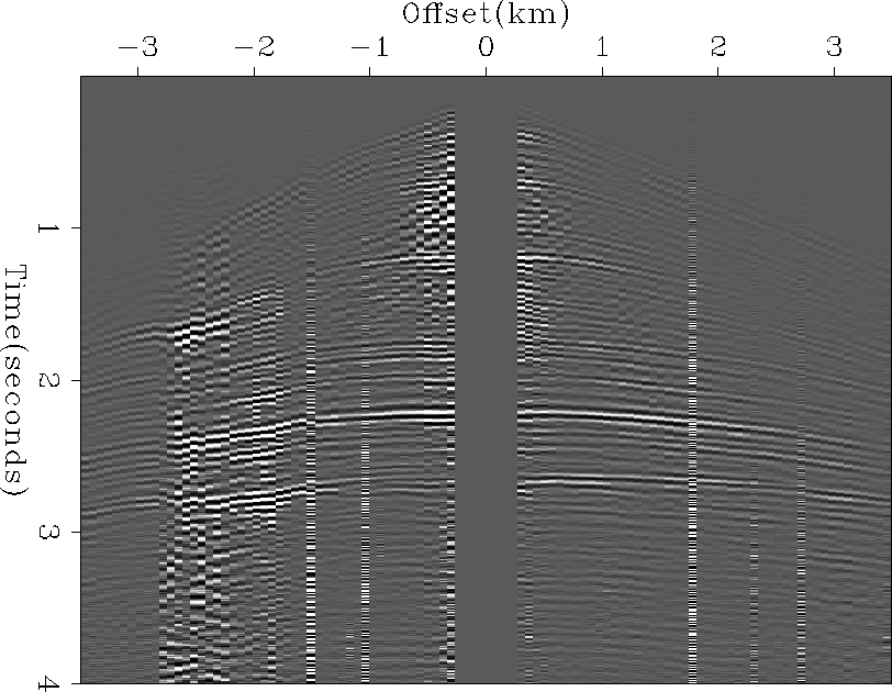
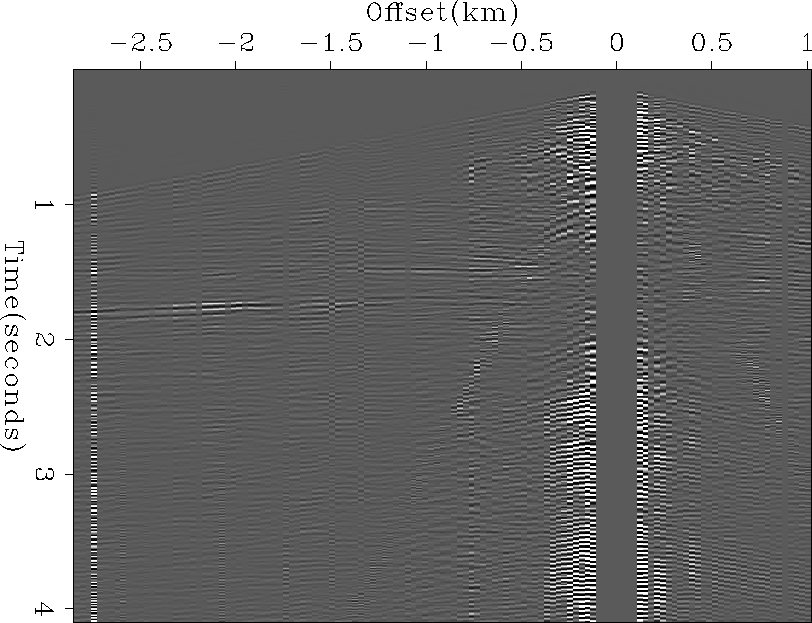
Figure ![[*]](http://sepwww.stanford.edu/latex2html/cross_ref_motif.gif) shows a shot gather with some obvious bad
traces.
The data here and in the following plots have been scaled
by time squared to show the signal better.
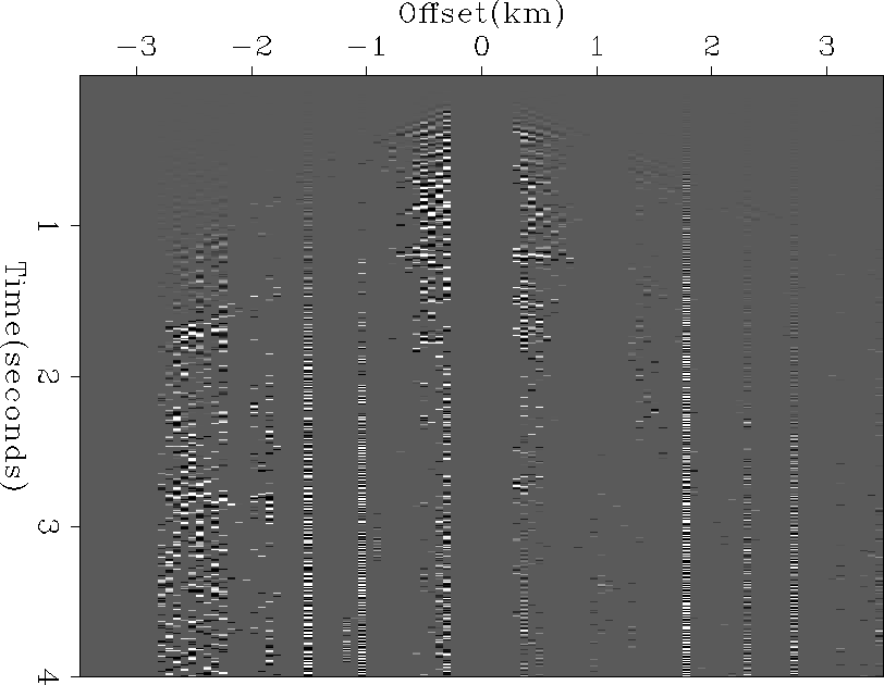
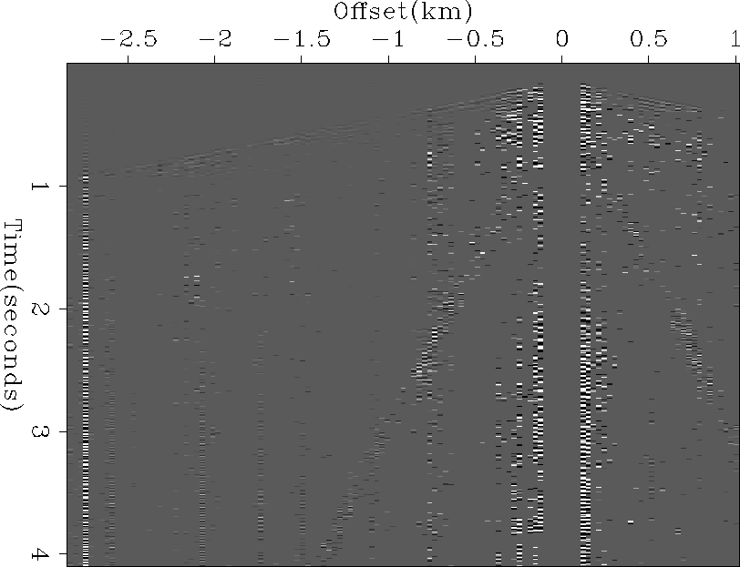
Figures and
shows the separation of the shot gather shown
in Figure into the rejected and the accepted
samples with a w of five.
In the electronic version of this thesis, pushing the button
under Figure shows a movie
of the data in this figure with a range of values of w.
For small values of w, for example 1 to 3,
the result of the process changed quickly from one value of w to another.
As w increased,
the changes in the results for different values of w decreased.
An example of a small portion of Figure processed with
values of w varying from 1 to 9 is shown in Figure .
shows a shot gather with some obvious bad
traces.
The data here and in the following plots have been scaled
by time squared to show the signal better.
Figures and
shows the separation of the shot gather shown
in Figure into the rejected and the accepted
samples with a w of five.
In the electronic version of this thesis, pushing the button
under Figure shows a movie
of the data in this figure with a range of values of w.
For small values of w, for example 1 to 3,
the result of the process changed quickly from one value of w to another.
As w increased,
the changes in the results for different values of w decreased.
An example of a small portion of Figure processed with
values of w varying from 1 to 9 is shown in Figure .
The result of this process appears to do a good job of removing
bad traces. Figure shows very little coherent signal
in the rejected samples.
The little coherent noise left in Figure appears on
the near traces, which have anomalous amplitudes.
 |


 |
![[*]](http://sepwww.stanford.edu/latex2html/movie.gif)
 |
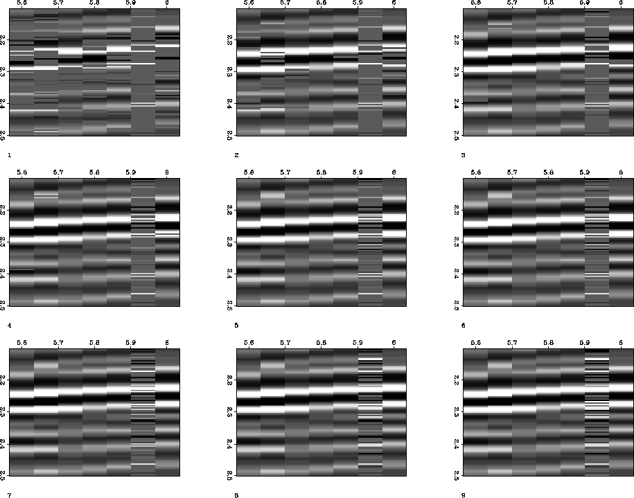 |
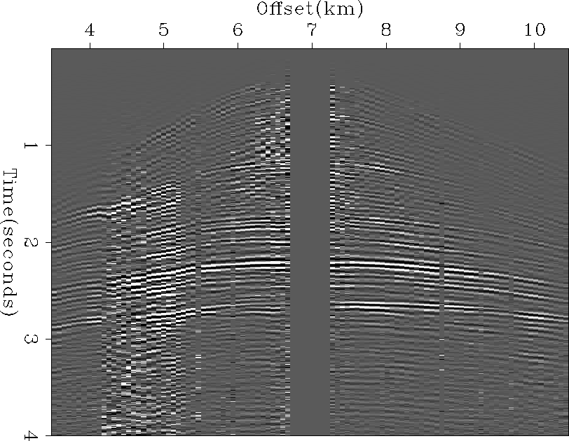
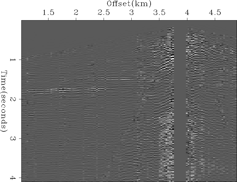
Figure shows another shot gather with some bad traces and some
coherent noise.
Once again,
the data here and in the following plots have been scaled
by time squared.
Figures and show that much of the coherent
noise between 2 and 3 seconds is removed.
This effect is seen here because the filters used to make the trace-to-trace
predictions are short, in this case five samples, and cannot predict much
of the steeply dipping energy.
While eliminating this particular event is desirable,
care must be taken to make the filters long enough to predict all
events that are to be preserved.
Events such as the diffractions from
complex events or overturned rays might not be predicted by very short
filters,
although generally these events will not be strong enough
to be thrown out.
In many cases, coherent noise is not as localized as it is in this
example and so will not be eliminated.
One advantage of this technique over similar methods is that, since predictions are done from single neighboring traces, static shifts do not affect the predictions. Both examples shown here have traces with static shifts that are passed without problems.
 |
 |
 |